`\color{green} ✍️` As we've studied, the inverse of a function `f,` denoted by `f^(–1),` exists if `f` is one-one and onto.

`\color{green} ✍️` As we know that trigonometric functions are not one-one and onto over their natural domains and ranges so their inverses do not exist.

`\color{green} ✍️` Here we will study, how to restrict domains and ranges of trigonometric functions which ensure the existence of their inverses.

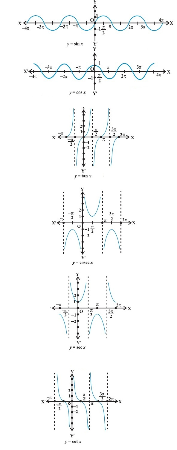
we have studied trigonometric functions, which are defined as follows:

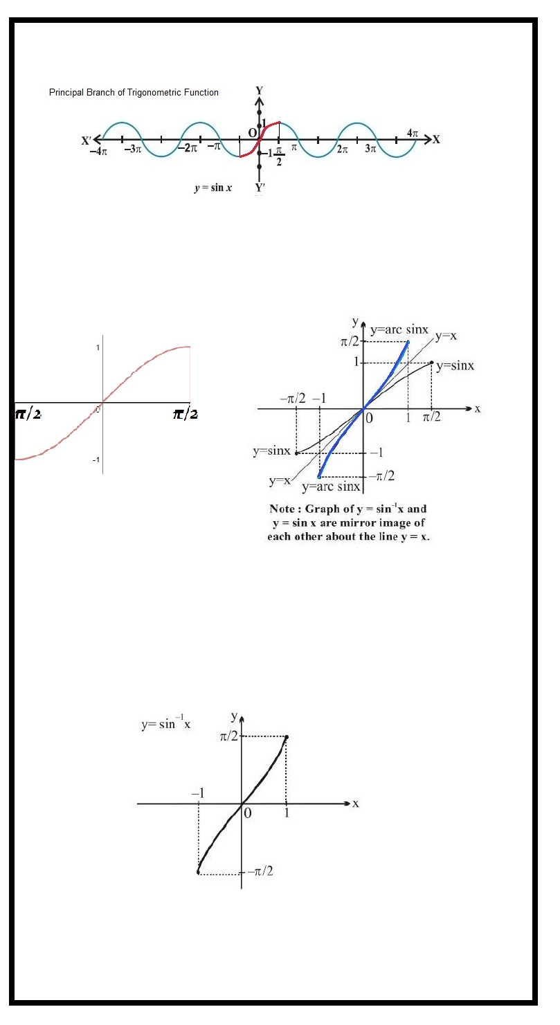
1. sine function, i.e.,
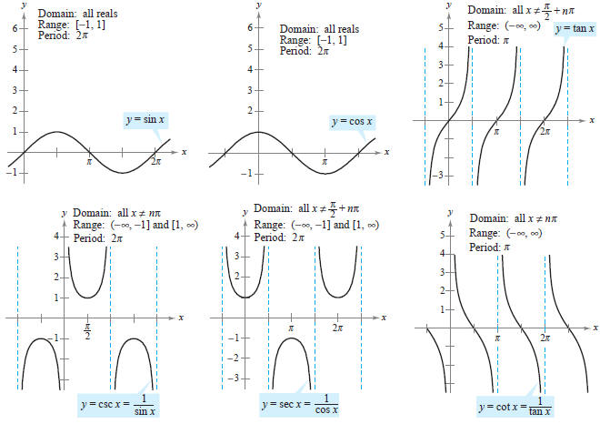
`sin : R → [– 1, 1]`

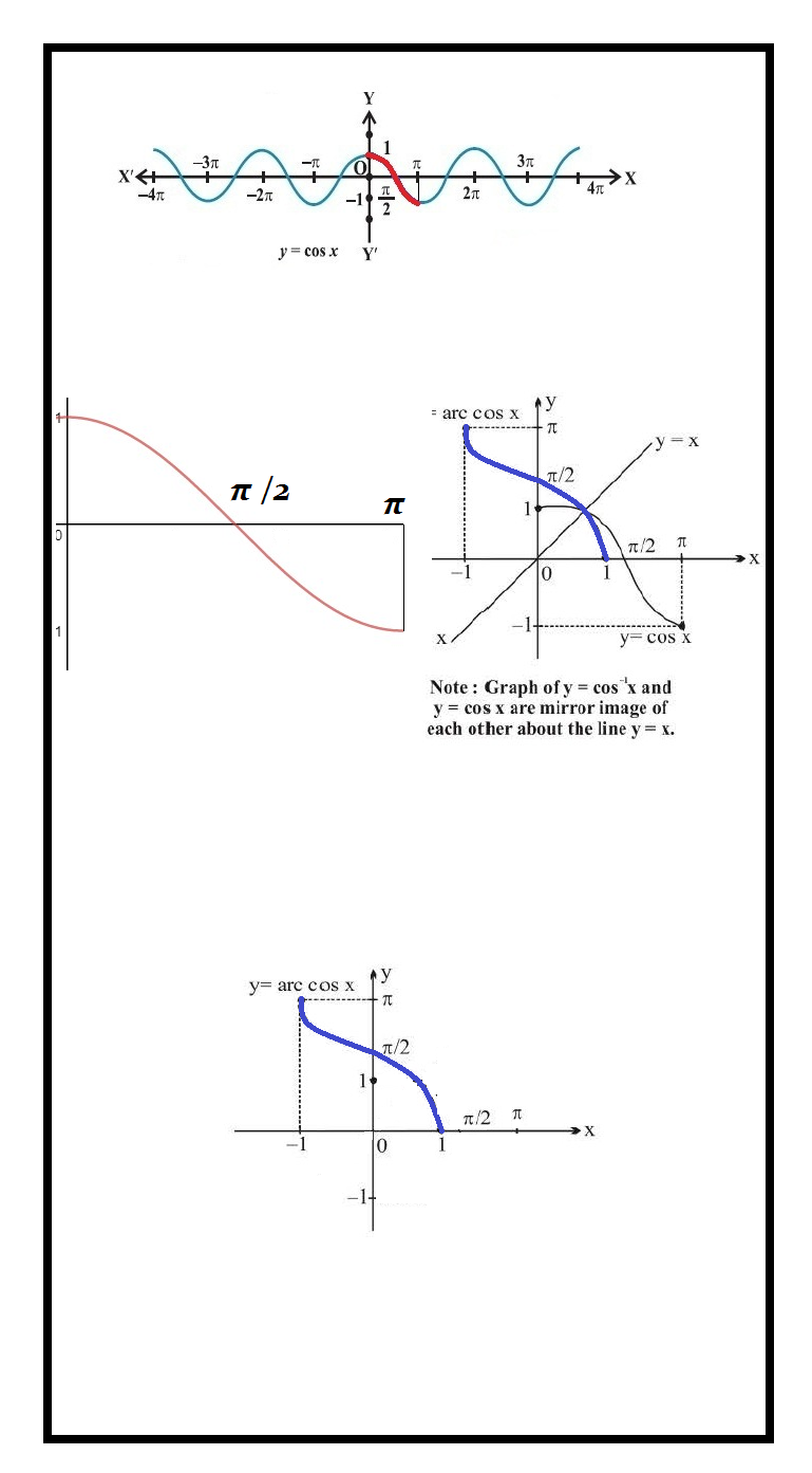
2. cosine function, i.e.,
` cos : R → [– 1, 1]`

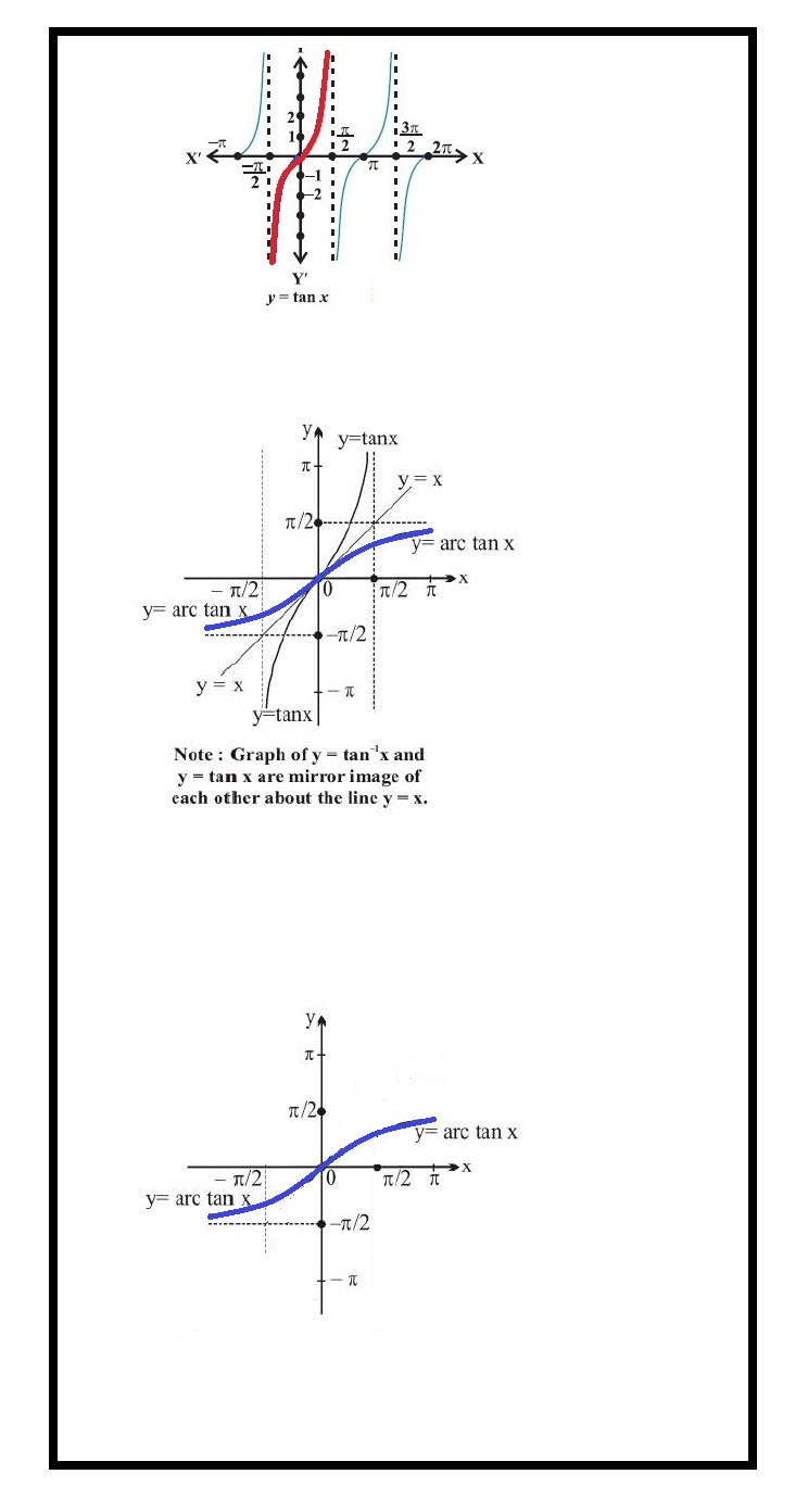
3. tangent function, i.e., `tan : R – { x : x = (2n + 1) π/2 , n ∈ Z} → R`

4. cotangent function, i.e.,
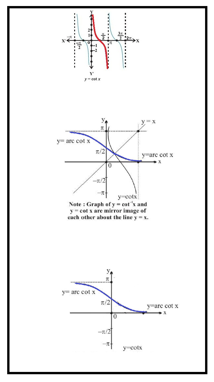
`cot : R – { x : x = nπ, n ∈ Z} → R`

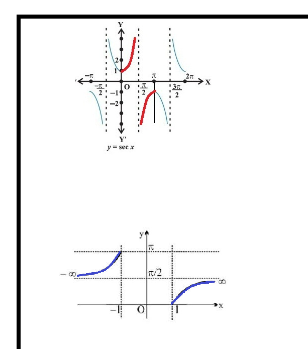
5.secant function, i.e., `sec : R – { x : x = (2n + 1)π/2 , n ∈ Z} → R – (– 1, 1)`

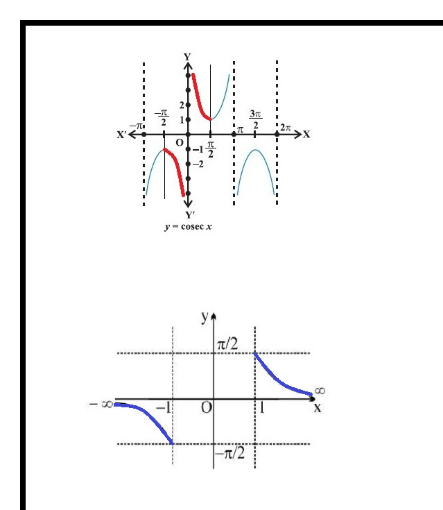
6. cosecant function, i.e., `cosec : R – { x : x = nπ, n ∈ Z} → R – (– 1, 1)`

`=>` Let us first take Sine function.

`y= sin x, quad quad R-> [-1,1]`

`=>` This function is not one-one and hence cannot be inverted.

But we can make a function one-one by restricting the domain.

`=>` We can make the function one-one by restricting the domain to `[-(3pi)/2 , -pi/2] , [ - pi/2 , pi/2] [ ( pi/2 , (3pi)/2]`

`\color{blue} ✍️ \color{green}(KEY \ CONCEPT) : ` The branch with range `[- \ pi/2 , pi/2]` is called principal value of branch, whereas other intervals as range give different branches of `sin^(–1)`.

`\color { maroon} ® \color{maroon} ul (" REMEMBER") :` Whenever we refer to the function `sin^(–1)`, we take it as the function whose domain is `[–1, 1]` and range is `[-pi/2,pi/2]`

`sin^(-1) : [-1 , 1]-> [ - \ pi/2 , pi/2]`

Remarks :

(i) If `y = f (x)` is an invertible function, then `x = f^(–1) (y)`. Thus, the graph of `sin^(–1)` function can be obtained from the graph of original function by interchanging `x` and `y` axes, i.e., if `(a, b)` is a point on the graph of sine function, then `(b, a)` becomes the corresponding point on the graph of inverse the graph of `y = sin x` by interchanging `x` and `y` axes. The graphs of `y = sin x` and `y = sin^(–1) x` are as given in . The dark portion of the graph of `y = sin^(–1) x` represent the principal value branch.

(ii) It can be shown that the graph of an inverse function can be obtained from the corresponding graph of original function as a mirror image (i.e., reflection) along the line `y = x`. This can be visualised by looking the graphs of `y = sin x` and `y = sin^(–1) x` as given in the same axes

`=>` Let us first take cos function, same as sin function

`y= cos x, quad quad R-> [-1,1]`

`=>` This function is not one-one and hence cannot be inverted.

But we can make a function one-one by restricting the domain.

`=>` We can make the function one-one by restricting the domain to `[- pi , 0] , [ 0 , pi] [ pi , 2pi]`

`\color{green} ✍️ \color{green} (KEY \ CONCEPT) : ` The branch with range `[0 , pi]` is called principal value of branch, whereas other intervals as range give different branches of `cos^(–1).`


`\color { maroon} ® \color{maroon} ul (" REMEMBER") :` Whenever we refer to the function `cos^(–1)`, we take it as the function whose domain is `[–1, 1]` and range is `[0,pi]`

`cos^(-1) : [-1 , 1]-> [ 0 , pi]`

`=>` Let us first take tan function,

`tan : R – { x : x = (2n + 1) π/2 , n ∈ Z} → R`

`=>` This function is not one-one and hence cannot be inverted.

But we can make a function one-one by restricting the domain.

`=>` We can make the function one-one by restricting the domain to `(- (3pi)/2 , -pi/2) , ( -pi/2 , pi/2), ( ( pi/2 , (3pi)/2))`

`\color{green} ✍️ \color{green} (KEY \ CONCEPT) : ` The branch with range `(-pi/2 , pi/2)` is called principal value of branch, whereas other intervals as range give different branches of `tan^(-1).`


`\color { maroon} ® \color{maroon} ul (" REMEMBER") :` Whenever we refer to the function `tan^(–1)`, we take it as the function whose domain is `R` and range is `(-pi/2,pi/2)`

`tan^(-1) : R-> ( -pi/2 , pi/2)`

`=>` Let us first take Sine function.

`cosec : R – { x : x = nπ, n ∈ Z} → R – (– 1, 1)`

`=>` This function is not one-one and hence cannot be inverted.

But we can make a function one-one by restricting the domain.

`=>` We can make the function one-one by restricting the domain to `[-(3pi)/2 , -pi/2] - {pi}, [ -pi/2 , pi/2] - {0}, [ pi/2 , (3pi)/2]-{pi}`

`\color{green} ✍️ \color{green} (KEY \ CONCEPT) : ` The branch with range `[- pi/2 , pi/2] - {0}` is called principal value of branch, whereas other intervals as range give different branches of `cosec^(–1).`


`\color { maroon} ® \color{maroon} ul (" REMEMBER") :` Whenever we refer to the function `cosec^(–1)`, we take it as the function whose domain is `R-[–1, 1]` and range is `[-pi/2,pi/2] - {0}`

`cosec^(-1) : R - [-1 , 1]-> [ - \ pi/2 , pi/2] - {0}`

`=>` Let us first take sec function,

`sec : R – { x : x = (2n + 1)π/2 , n ∈ Z} → R – (– 1, 1)`

`=>` This function is not one-one and hence cannot be inverted.

But we can make a function one-one by restricting the domain.

`=>`We can make the function one-one by restricting the domain to `[- pi , 0]-{-pi/2} , [ 0 , pi]-{pi/2}, [ pi , 2pi] - {(3pi)/2}`

`\color{green} ✍️ \color{green} (KEY \ CONCEPT) : ` The branch with range `[0 , pi] - {pi/2}` is called principal value of branch, whereas other intervals as range give different branches of `sec^(–1).`


`\color { maroon} ® \color{maroon} ul (" REMEMBER") :` Whenever we refer to the function `sec^(–1)`, we take it as the function whose domain is `R - [–1, 1]` and range is `[0,pi]-{pi/2}`

`sec^(-1) :R- [-1 , 1]-> [ 0 , pi]-{pi/2}`

`=>` Let us first take cot function, same as sin function

`cot : R - { x : x = nπ, n ∈ Z} → R`

`=>` This function is not one-one and hence cannot be inverted.

But we can make a function one-one by restricting the domain.

`=>` We can make the function one-one by restricting the domain to `(- pi , 0) , ( 0 , pi), ( pi , 2pi)`

`\color{green} ✍️ \color{green} (KEY \ CONCEPT) : ` The branch with range `(0 , pi)` is called principal value of branch, whereas other intervals as range give different branches of `cot^(–1).`


`\color { maroon} ® \color{maroon} ul (" REMEMBER") :` Whenever we refer to the function `cot^(–1)`, we take it as the function whose domain is `R` and range is `(0,pi)`

`cot^(-1) : R -> (0 , pi)`