Physics ELECTRIC FIELDS AND ELECTRIC FLUX

TOPIC COVERED

`color{blue}{star}` Forces Between Multiple Charges
`color{blue}{star}` Electric Field
`color{blue}{star}` Electric Field Lines
`color{blue}{star}` Electric Flux

FORCES BETWEEN MULTIPLE CHARGES

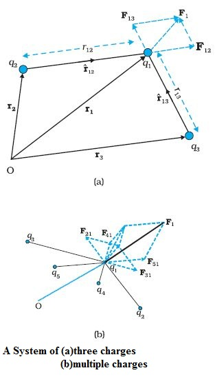
`color {blue}✍️ ` Consider a system of three charges ` q_1`, `q_2` and `q_3`.

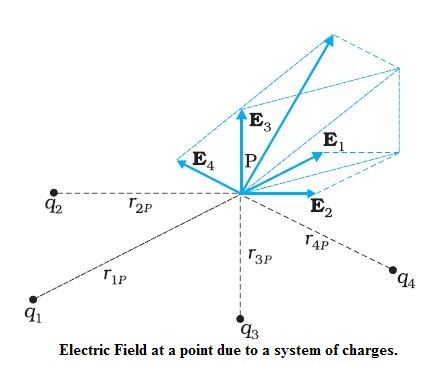
The force on charge` q_1`, due to two other charges `q_2`, `q_3` can be obtained by performing a vector addition of the forces due to each one of these charges. Thus, if the force on `q_1` due to `q_2` is denoted by `vec F_(12)`,

`vec F_(12)=1/(4πε_0)((q_1q_2)/r_(12)^2)hat r_(12)`

The force on `q_1` due to `q_3`, denoted by `vec F_13`, is given by

`vec F_(13)=1/(4πε_0)((q_1q_3)/r_(13)^2)hat r_(13)`

which is the Coulomb force on `q_1` due to `q_3`

Thus the total force`vec F_1` on `q_1` due to the two charges `q_2` and `q_3` is given as :

`vec F_1 = vec F_(12) +vec F_(13) =1/(4πε_0)((q_1q_2)/r_(12)^2)hat r_(12)+1/(4πε_0)((q_1q_3)/r_(13)^2)hat r_(13)`

The principle of superposition says that in a system of charges `q_1, q_2, ..., q_n`, the force on `q_1` due to `q_2` is the same as given by Coulomb’s law, i.e., it is unaffected by the presence of the other charges `q_3, q_4, ..., q_n`.

The total force `vec F_1` on the charge `q_1`, due to all other charges, is then given by the vector sum of the forces `vec F_(12), vec F_(13), ...,vec F_(1n)`:

`\color{red}ul(★ \color{red} " FORMULA ALERT")`

`vec F_1 = vec F_(12) +vec F_(13) + ...... +vec F_(1n)`

` =1/(4πε_0)[(q_1q_2)/r_(12)^2hat r_(12)+(q_1q_3)/r_(13)^2hat r_(13) +............ +(q_1q_n)/r_(1n)^2hat r_(1n)]`

`=q_1/(4πε_0)sum_(i=2)^(n)q_i/r_(1i)^2hat r_(1i)`

The vector sum is obtained by the parallelogram law of addition of vectors.
Q 3220680511

Consider three charges `q_1, q_2 , q_3` each equal to `q` at the vertices of an equilateral triangle of side `l`. What is the force on a charge `Q` (with the same sign as `q`) placed at the centroid of the triangle, as shown in Fig. 1.9?
Class Chapter 1 Example 6
Solution:

In the given equilateral triangle `ABC` of sides of length `l`, if we draw a perpendicular `AD` to the side `BC`, `AD = AC cos 30º = ( sqrt(3)//2 ) l` and the distance `AO` of the centroid `O` from `A` is `(2//3) AD = (1// sqrt(3 )) l`. By symmatry `AO = BO = CO`

Thus,
Force `F_1` on `Q` due to charge `q` at `A = 3/( 4 π ε_0)` `(Qq)/l^2` along `AO`

Force ` F_2` on `Q` due to charge `q` at `B = 3/( 4 π ε_0)` `(Qq)/l^2` along `BO`

Force `F_3` on `Q` due to charge `q` at `C = 3/( 4 π ε_0)` `(Qq)/l^2` along `CO`

The resultant of forces `F_2` and `F_3` is `3/( 4 π ε_0)` `(Qq)/l^2` along `OA` by the parallelogram law. Therefore, the total force on `Q = 3/( 4 π ε_0)` `(Qq)/i^2 (hat r - hat r)`

`= O`, where `hat r` is the unit vector along `OA`.
It is clear also by symmetry that the three forces will sum to zero.
Suppose that the resultant force was non-zero but in some direction.
Consider what would happen if the system was rotated through `60º` about `O`.
Q 3230680512

Consider the charges `q, q,` and `–q` placed at the vertices of an equilateral triangle, as shown in Fig. 1.10. What is the force on each charge?
Class Chapter 1 Example 7
Solution:

The forces acting on charge `q` at `A` due to charges `q` at `B`
and `–q` at `C` are `F_(12)` along `BA` and `F_(13)` along `AC` respectively, as shown
in Fig. 1.10. By the parallelogram law, the total force `F_1` on the charge
`q` at `A` is given by
`F_1 = F hat r_1` where `hat r_1` is a unit vector along `BC`.
The force of attraction or repulsion for each pair of charges has the

same magnitude ` F = q^2/(4 pi ε_0 l^2)`

The total force `F^2` on charge `q` at `B` is thus `F_2 = F hat r_2`, where `hat r_2` is a
unit vector along `AC`.

Similarly the total force on charge `–q` at `C` is `F_3 = sqrt 3 F hat n` , where `hat n` is
the unit vector along the direction bisecting the `∠BCA`.
It is interesting to see that the sum of the forces on the three charges
is zero, i.e.,

`F_1 + F_2 + F_3 = 0`

The result is not at all surprising. It follows straight from the fact that Coulomb’s law is consistent with Newton’s third law. The proof is left to you as an exercise.

Electric Field

Let us consider a point charge `Q` placed in vacuum, at the origin `O`.

Another point charge q at a point P, where `OP = r`, then the charge Q will exert a force on `q` as per Coulomb’s law.

When another charge `q` is brought at some point P, the field there acts on it and produces a force. The electric field produced by the charge `Q` at a point `r` is given as

`vec F(vec r) = 1/(4πε_0)q/(r^2)hat r`

where `hat r =vec r/r`, is a unit vector from the origin to the point `r`.

`\color{blue} ✍️` The above equation specifies the value of the electric field for each value of the position vector `r`.

`color{blue}●`The word “field” signifies how some distributed quantity (which could be a scalar or a vector) varies with position.

`color{blue}●`The effect of the charge has been incorporated in the existence of the electric field. We obtain the force `F` exerted by a charge `Q` on a charge `q`, as

`vec F= 1/(4πε_0)(Qq)/r^2 hatr`

`color{blue}{1.}` The charge `q` also exerts an equal and opposite force on the charge `Q` .

`color{blue}{2.}` The electrostatic force between the charges `Q` and ` q` can be looked upon as an interaction between charge `q` and the electric field of ` Q` and vice versa.

`color{blue}{3.}` If we denote the position of charge` q` by the vector ` r`, it experiences a force` F` equal to the charge ` q ` multiplied by the electric field `E` at the location of `q` .

`vec F(vec r) = q vec E(vec r) `

The SI unit of electric field as` N/C` .

`\color{blue} ✍️` Some important remarks made here:

`color{blue}{(i)}`The electric field due to a charge `Q` at a point in space may be defined as the force that a unit positive charge would experience if placed at that point.

`color{blue}●` The charge `Q` , which is producing the electric field, is called a `"source charge"`.

`color{blue}●` The charge` q`, which tests the effect of a source charge, is called a `"test charge"`.

`color{blue}●`The force `F `is then negligibly small but the ratio` F/q` is finite and defines the electric field:

`E= lim_(q->0)(F/Q)`

`color{blue}{(ii)}` The ratio `F/q ` does not depend on `q`.

`color{blue}●`The electric field `E` due to ` Q `is also dependent on the space coordinate r.

`color{blue}●`The field exists at every point in three-dimensional space.

`color{blue}{(iii)}` For a positive charge, the electric field will be directed radially outwards from the charge.

`color{blue}{(iv)}` For negative, the electric field vector, at each point, points radially inwards.

`color{blue}{(v)}` The magnitude of the electric field` E` will also depend only on the distance` r` .

Electric Field due to a System of Charges

Consider a system of charges `q_1`, `q_2`, ..., `q_n` with position vectors `r_1`, `r_2`, ..., `r_n` relative to some origin O. Electric field at a point in space due to the system of charges is defined to be the force experienced by a unit test charge placed at that point, without disturbing the original positions of charges `q_1`, `q_2`, ..., `q_n`.

`color{blue}●` By using Coulomb’s law and the superposition principle to determine this field at a point `P` denoted by position vector `r`.

`\color{blue} ✍️`Electric field `E_1` at r due to `q_1` at `r_1` is given by

` E_1=1/(4πε_0)q_1/r_(1P)^2 hat r_(1P)`

where
`hat r _(1P)` is a unit vector in the direction from `q_1` to P ,
`r_(1P)` is the distance between `q_1` and P .

`\color{blue} ✍️`Electric field `E_2` at r due to `q_2` at

` E_2=1/(4πε_0)q_2/r_(2P)^2 hat r_(2P)`

where
`hat r_(2P)` is a unit vector in the direction from `q_2` to P,

` r_(2P)` is the distance between `q_2` and P.

Similar expressions for fields `E_3`, `E_4`, ..., `E_n` due to charges `q_3`, `q_4`, ..., `q_n`.

`\color{blue} ✍️`By the superposition principle, the electric field E at r due to the system of charges is

`E(r) = E_1 (r) + E_2 (r) + … + E_n(r)`

`=1/(4πε_0)q_1/r_(1P)^2 hat r_(1P)+1/(4πε_0)q_2/r_(2P)^2 hat r_(2P)+......+1/(4πε_0)q_n/r_(nP)^2 hat r_(nP)`

`E(r)=1/(4πε_0)sum_(i=1)^(n)q_i/r_(iP)^2 hat r_(iP)`

`E` is a vector quantity that varies from one point to another point in space and is determined from the positions of the source charges.

Physical significance of electric field

The physical significance of the concept of electric field, emerges only when we go beyond electrostatics and deal with time dependent
electromagnetic phenomena.

`color{blue}✍️` Suppose we consider the force between two distant charges `q_1`, `q_2` in accelerated motion. Now the greatest speed with which a signal or information can go from one point to another is c, the speed of light.

`color{blue}✍️` The accelerated motion of charge `q_1` produces electromagnetic waves, which then propagate with the speed `c`, reach `q_2` and cause a force on `q_2`.

`color{blue}✍️` Electric field have an independent dynamics of their own, i.e., they evolve according to laws of their own.

`color{blue}✍️` They can also transport energy.
Q 3240680513

An electron falls through a distance of `1.5 cm` in a uniform electric field of magnitude `2.0 xx 10^4 N C^(–1)` [Fig. 1.13(a)]. The direction of the field is reversed keeping its magnitude unchanged and a proton falls through the same distance [Fig. 1.13(b)]. Compute the time of fall in each case. Contrast the situation with that of ‘free fall under gravity’.
Class Chapter 1 Example 8
Solution:

In Fig. 1.13(a) the field is upward, so the negatively charged
electron experiences a downward force of magnitude `eE` where `E` is
the magnitude of the electric field. The acceleration of the electron is

`a_e = eE//m_e`

where me is the mass of the electron.

Starting from rest, the time required by the electron to fall through a
distance h is given by ` t_e = sqrt( (2h)/a_e) = sqrt ((2h m_e)/(eE))`

For `e = 1.6 xx 10^(–19) C, m_e = 9.11 xx 10^(–31) kg`,

`E = 2.0 xx 10^4 N C^(–1) , h = 1.5 xx 10^(–2) m`,

`t_e = 2.9 xx 10^(–9) s`

In Fig. 1.13 (b), the field is downward, and the positively charged
proton experiences a downward force of magnitude `eE`. The
acceleration of the proton is

`a_p = eE//m_p`

where `m_p` is the mass of the proton; `m_p = 1.67 xx 10^(–27) kg`. The time of
fall for the proton is

` t_p = sqrt( (2h)/a_p) = sqrt ((2h m_p)/(eE)) = 1.3 xx 10^(-7) s`

Thus, the heavier particle (proton) takes a greater time to fall through
the same distance. This is in basic contrast to the situation of ‘free
fall under gravity’ where the time of fall is independent of the mass of
the body. Note that in this example we have ignored the acceleration
due to gravity in calculating the time of fall. To see if this is justified,
let us calculate the acceleration of the proton in the given electric
field:

` a_p = (eE)/m_p`

` = ( (1 .6 xx 10^(-19) C) xx (2. 0 xx 10^4 N C^(-1) ))/( 1.67 xx 10^(-27) kg)`

` = 1.9 xx 10^(12) ms^(-2)`

which is enormous compared to the value of g `(9.8 m s^(–2) )`, the
acceleration due to gravity. The acceleration of the electron is even
greater. Thus, the effect of acceleration due to gravity can be ignored
in this example.
Q 3260680515

Two point charges `q_1` and `q_2`, of magnitude `+10^(–8) C` and
`–10^(–8) C`, respectively, are placed `0.1 m` apart. Calculate the electric
fields at points `A, B` and `C` shown in Fig. 1.14.
Class Chapter 1 Example 9
Solution:

The electric field vector `E_(1A)` at A due to the positive charge
`q_1` points towards the right and has a magnitude

`E_(1A) = ( (9 xx 10^9 N m^2 C^(-2) ) xx (10^(-8) C ))/( 0.05m)^2 = 3.6 xx 10^4 N C^(–1)`

The electric field vector `E_(2A)` at A due to the negative charge `q_2` points
towards the right and has the same magnitude. Hence the magnitude
of the total electric field `E_A` at A is
`E_A = E_(1A) + E_(2A) = 7.2 xx 10^4 N C^(–1)`

`E_A` is directed toward the right

The electric field vector `E_(1B)` at `B` due to the positive charge `q_1` points
towards the left and has a magnitude

` E_(1B) = ( (9 xx 10^9 N m^2 C^(-2) ) xx (10^8 C))/(0.05m)^2 = 3.6 xx 10^4 N C^(–1)`

The electric field vector `E_(2B)` at `B` due to the negative charge `q_2` points
towards the right and has a magnitude

` E_(2B) = ( (9 xx 10^9 Nm^2 C^(-2) ) xx (10^(-8) C))/( 0.05m)^2 = 4 xx 10^3 N C^(–1)`

The magnitude of the total electric field at B is

`E_B = E_(1B) – E_(2B) = 3.2 xx 10^4 N C^(–1)`

`E_B` is directed towards the left.

The magnitude of each electric field vector at point C, due to charge
`q_1` and `q_2` is

`E_(1C) = E_(2C) = ( (9 xx 10^9 Nm^2 C^(-2) ) xx (10^(-8) C))/( 0.10 m)^2 = 9 xx 10^3 N C^(–1)`

The directions in which these two vectors point are indicated in
Fig. 1.14. The resultant of these two vectors is

` E_c = E_1 cos pi/3 + E_2 cos pi/3 = 9 xx 10^3 N C^(–1)`

`E_c` points towards the right.

ELECTRIC FIELD LINES

`color{blue}✍️` `E` is strong near the charge, so the density of field lines is more near the charge and the lines are closer. Away from the charge, the field gets weaker and the density of field lines is less, resulting in well-separated lines.


`color{blue}✍️` The field lines of a single positive charge are radially outward while those of a single negative charge are radially inward. The field lines around a system of two positive charges (q, q) give a vivid pictorial description of their mutual repulsion, while those around the configuration of two equal and opposite charges (q,–q), a dipole, show clearly the mutual attraction between the charges.

`color{blue}✍️` The field lines follow some important general properties:


`color{blue}{ (i)}` Field lines start from positive charges and end at negative charges. If there is a single charge, they may start or end at infinity.

`color{blue}{(ii)}` In a charge-free region, electric field lines can be taken to be continuous curves without any breaks.

`color{blue}{(iii)}` Two field lines can never cross each other.

`color{blue}{(iv)}` Electrostatic field lines do not form any closed loops.

ELECTRIC FLUX

Electric flux `Δφ` through an area element `ΔS` is defined by:

`Δφ = E.ΔS = E ΔS cosθ`

which, is proportional to

`color{blue}{1.}` The number of field lines cutting the area element.

`color{blue}{2.}` The angle θ here is the angle between `E` and `ΔS`.

`\color{blue} ✍️` `θ` is the angle between E and the outward normal to the area element.

The unit of electric flux is `N C^(–1) m^2`.

To calculate the total flux through any given surface. All we have to do is to divide the surface into small area elements, calculate the
flux at each element and add them up. Thus, the total flux `φ` through a surface `S` is

`φ ~ Σ E.ΔS `

The approximation sign is put because the electric field E is taken to be constant over the small area element. This is mathematically exact only when you take the limit `ΔS → 0` and the sum is written as an integral.

 
SiteLock