EQUIPOTENTIAL SURFACES
`color{blue} ✍️` An equipotential surface is a surface with a constant value of potential at all points on the surface.
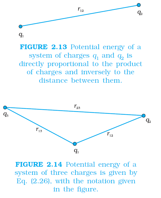
`color{blue} ✍️` For a single charge `q,` the potential is given by Eq. (2.8):
`color{blue} {V = 1/(4piepsilon_0) q/r}`
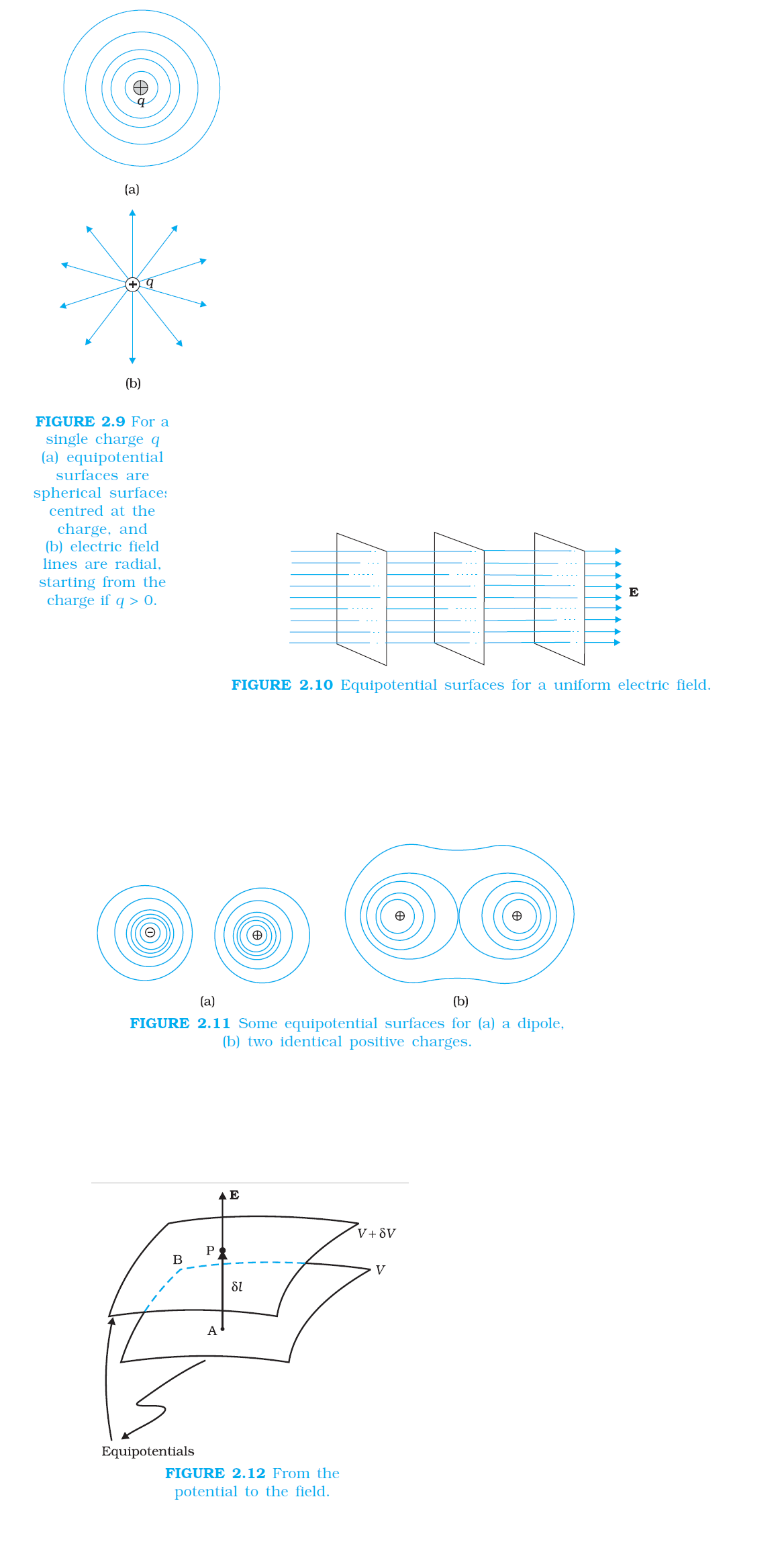
`color{blue} ✍️` This shows that `V` is a constant if `r` is constant . Thus, equipotential surfaces of a single point charge are concentric spherical surfaces centred at the charge.
`color{blue} ✍️` Now the electric field lines for a single charge `q` are radial lines starting from or ending at the charge, depending on whether `q` is positive or negative.
`color{blue} ✍️` Clearly, the electric field at every point is normal to the equipotential surface passing through that point. This is true in general for any charge configuration, equipotential surface through a point is normal to the electric field at that point.
`color{blue} ✍️` The proof of this statement is simple. If the field were not normal to the equipotential surface, it would have non-zero component along the surface.
`color{blue} ✍️` To move a unit test charge against the direction of the component of the field, work would have to be done.
`color{blue} ✍️` But this is in contradiction to the definition of an equipotential surface: there is no potential difference between any two points on the surface and no work is required to move a test charge on the surface.
`color{blue} ✍️` The electric field must, therefore, be normal to the equipotential surface at every point. Equipotential surfaces offer an alternative visual picture in addition to the picture of electric field lines around a charge configuration.

`color{blue} ✍️` For a uniform electric field E, say, along the x -axis, the equipotential surfaces are planes normal to the x -axis, i.e., planes parallel to the y-z plane (Fig. 2.10). Equipotential surfaces for (a) a dipole and (b) two identical positive charges are shown in Fig. 2.11.

`color{blue}ulbb "Relation between field and potential"`
`color{blue} ✍️` Consider two closely spaced equipotential surfaces A and B (Fig. 2.12) with potential values `V` and `V + δV,` where `δV` is the change in `V` in the direction of the electric field `E.`
`color{blue} ✍️` Let `P` be a point on the surface `B`. `δl` is the perpendicular distance of the surface A from `P`. Imagine that a unit positive charge is moved along this perpendicular from the surface B to surface A against the electric field. The work done in this process is `|E|δ l.`

`color{blue} ✍️` This work equals the potential difference `V_A–V_B`
Thus,
`|E|δ l = V−(V +δV)= –δV`
i.e., `color{blue} {|E|= (δV)/(δ l)}` .................... 2.20
Since `δV` is negative, `δV = – |δV|.` we can rewrite Eq (2.20) as
`color{blue} ✍️` We thus arrive at two important conclusions concerning the relation between electric field and potential:
`color{blue} ✍️` Electric field is in the direction in which the potential decreases steepest.
`color{blue} ✍️` Its magnitude is given by the change in the magnitude of potential per unit displacement normal to the equipotential surface at the point.
`color{blue} ✍️` For a single charge `q,` the potential is given by Eq. (2.8):
`color{blue} {V = 1/(4piepsilon_0) q/r}`
`color{blue} ✍️` This shows that `V` is a constant if `r` is constant . Thus, equipotential surfaces of a single point charge are concentric spherical surfaces centred at the charge.
`color{blue} ✍️` Now the electric field lines for a single charge `q` are radial lines starting from or ending at the charge, depending on whether `q` is positive or negative.
`color{blue} ✍️` Clearly, the electric field at every point is normal to the equipotential surface passing through that point. This is true in general for any charge configuration, equipotential surface through a point is normal to the electric field at that point.
`color{blue} ✍️` The proof of this statement is simple. If the field were not normal to the equipotential surface, it would have non-zero component along the surface.
`color{blue} ✍️` To move a unit test charge against the direction of the component of the field, work would have to be done.
`color{blue} ✍️` But this is in contradiction to the definition of an equipotential surface: there is no potential difference between any two points on the surface and no work is required to move a test charge on the surface.
`color{blue} ✍️` The electric field must, therefore, be normal to the equipotential surface at every point. Equipotential surfaces offer an alternative visual picture in addition to the picture of electric field lines around a charge configuration.
`color{blue} ✍️` For a uniform electric field E, say, along the x -axis, the equipotential surfaces are planes normal to the x -axis, i.e., planes parallel to the y-z plane (Fig. 2.10). Equipotential surfaces for (a) a dipole and (b) two identical positive charges are shown in Fig. 2.11.
`color{blue}ulbb "Relation between field and potential"`
`color{blue} ✍️` Consider two closely spaced equipotential surfaces A and B (Fig. 2.12) with potential values `V` and `V + δV,` where `δV` is the change in `V` in the direction of the electric field `E.`
`color{blue} ✍️` Let `P` be a point on the surface `B`. `δl` is the perpendicular distance of the surface A from `P`. Imagine that a unit positive charge is moved along this perpendicular from the surface B to surface A against the electric field. The work done in this process is `|E|δ l.`
`color{blue} ✍️` This work equals the potential difference `V_A–V_B`
Thus,
`|E|δ l = V−(V +δV)= –δV`
i.e., `color{blue} {|E|= (δV)/(δ l)}` .................... 2.20
Since `δV` is negative, `δV = – |δV|.` we can rewrite Eq (2.20) as
`color{blue}{|E|= (δV)/(δ l) = + (|δV|)/(δ l)}`
.....................2.21`color{blue} ✍️` We thus arrive at two important conclusions concerning the relation between electric field and potential:
`color{blue} ✍️` Electric field is in the direction in which the potential decreases steepest.
`color{blue} ✍️` Its magnitude is given by the change in the magnitude of potential per unit displacement normal to the equipotential surface at the point.