`color{blue} ✍️` The Danish physicist Hans Christian Oersted noticed that a current in a straight wire caused a noticeable deflection in a nearby magnetic compass needle.

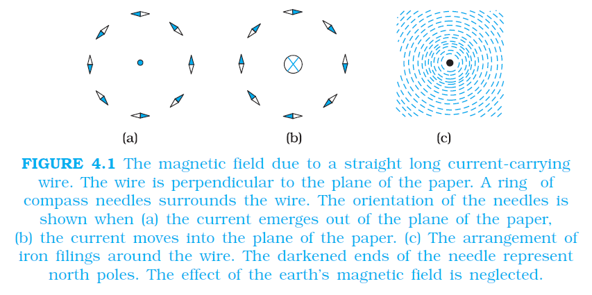
`color{blue} ✍️` He found that the alignment of the needle is tangential to an imaginary circle which has the straight wire as its centre and has its plane perpendicular to the wire.

`color{blue} ✍️` This situation is depicted in Fig.4.1(a). It is noticeable when the current is large and the needle sufficiently close to the wire so that the earth’s magnetic field may be ignored. Reversing the direction of the current reverses the orientation of the needle [Fig. 4.1(b)].

`color{blue} ✍️` The deflection increases on increasing the current or bringing the needle closer to the wire. Iron filings sprinkled around the wire arrange themselves in concentric circles with the wire as the centre [Fig. 4.1(c)].

`color{blue} ✍️` Obersted concluded that moving charges or currents produced a magnetic field in the surrounding space.

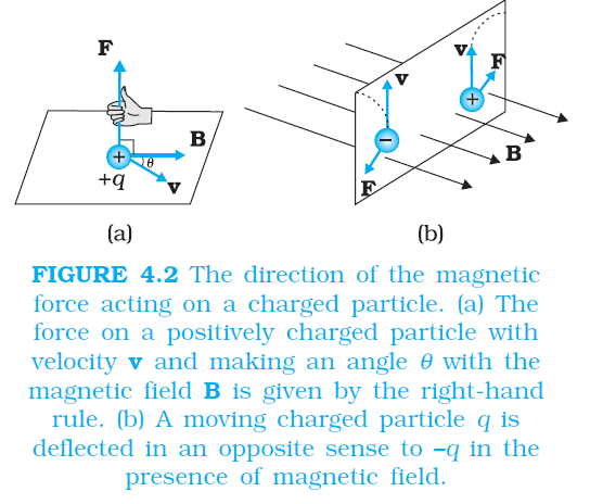
`color{blue} ✍️` In this chapter, we will see how magnetic field exerts forces on moving charged particles, like electrons, protons, and current-carrying wires.

`color{blue} ✍️` We shall also learn how currents produce magnetic fields. We shall see how particles can be accelerated to very high energies in a cyclotron. We shall study how currents and voltages are detected by a galvanometer. In this and subsequent

`color{blue} ✍️` Chapter on magnetism, we adopt the following convention: A current or a field (electric or magnetic) emerging out of the plane of the paper is depicted by a dot (⊚). A current or a field going into the plane of the paper is depicted by a cross (⊗)*. Figures. 4.1(a) and 4.1(b) correspond to these two situations, respectively.

`color{brown}bbul{"Sources and fields"}`
`color{blue} ✍️` As We have seen that the interaction between two charges can be considered in two stages. The charge `Q`, the source of the field, produces an electric field `E`, where

`color{navy}(E = Q hatr / {(4πε_0)r^2} ..........(4.1))`

`color {blue}➢` where `hatr` is unit vector along `r`, and the field `E` is a vector field. A charge q interacts with this field and experiences `ma` force `F` given by

`color{navy}(F = q E = (q Q hat r) / {(4πε_0) r^2} ............(4.2))`

`color{blue} ✍️` As pointed out the field `E` is not just an artefact but has a physical role. It can convey energy and momentum and is not established instantaneously but takes finite time to propagate.

`color{blue} ✍️` The concept of a field was specially stressed by Faraday and was incorporated by Maxwell in his unification of electricity and magnetism.

`color{blue} ✍️` In addition to depending on each point in space, it can also vary with time, i.e., be a function of time. In our discussions in this chapter, we will assume that the fields do not change with time.

`color{blue} ✍️` The field at a particular point can be due to one or more charges. If there are more charges the fields add vectorially.

`color{blue} ✍️` Once the field is known, the force on a test charge is given by Eq. (4.2). Just as static charges produce an electric field, the currents or moving charges produce (in addition) a magnetic field, denoted by `B (r)`, again a vector field.

`color{blue} ✍️` It has several basic properties identical to the electric field. It is defined at each point in space (and can in addition depend on time). Experimentally, it is found to obey the principle of superposition: the magnetic field of several sources is the vector addition of magnetic field of each individual source.

`color{blue} ✍️` Let us suppose that there is a point charge `q` (moving with a velocity `v` and, located at `r` at a given time `t` ) in presence of both the electric field `E (r)` and the magnetic field `B (r)`. The force on an electric charge q due to both of them can be written as

`color{navy}(F = q [ E (r) + v × B (r)] ≡ F_("electric") +F_("magnetic")).........(4.3)`

`color{blue} ✍️` This force was given first by H.A. Lorentz based on the extensive experiments of Ampere and others. It is called the Lorentz force.

`color{blue} ✍️` You have already studied in detail the force due to the electric field. If we look at the interaction with the magnetic field, we find the following features.

`color{blue} {(i)}` It depends on `q, v` and `B` (charge of the particle, the velocity and the magnetic field). Force on a negative charge is opposite to that on a positive charge.

`color{blue} {(ii)}` The magnetic force `q [ v × B ]` includes a vector product of velocity and magnetic field. The vector product makes the force due to magnetic field vanish (become zero) if velocity and magnetic field are parallel or anti-parallel. The force acts in a (sideways) direction perpendicular to both the velocity and the magnetic field. Its direction is given by the screw rule or right hand rule for vector (or cross) product as illustrated in Fig. 4.2.

`color{blue} ✍️{ (iii)}` The magnetic force is zero if charge is not moving (as then `|v|= 0`). Only a moving charge feels the magnetic force. The expression for the magnetic force helps us to define the unit of the magnetic field, if one takes `q, F` and `v`, all to be unity in the force equation

`color{navy}(F = q [ v × B] =q v B sin θ hat n)`

`color {blue}➢` where `θ` is the angle between `v` and `B` [see Fig. 4.2 (a)].

`color{blue} ✍️` The magnitude of magnetic field B is `1 SI` unit, when the force acting on a unit charge `(1 C)`, moving perpendicular to `B` with a speed `1m//s,` is one newton.

Dimensionally, we have `[B] = [F//qv]` and the unit of `B` are Newton second / (coulomb metre).

`color{blue} ✍️` This unit is called tesla (`T`) named after Nikola Tesla (1856 – 1943). Tesla is a rather large unit. A smaller unit (non-SI) called gauss (=`10^(–4)` tesla) is also often used. The earth’s magnetic field is about `(3.6 × 10^(–5) T.)`

`color{blue} ✍️` Table 4.1 lists magnetic fields over a wide range in the universe.

`color{blue} ✍️` We can extend the analysis for force due to magnetic field on a single moving charge to a straight rod carrying current.

`color{blue} ✍️` Consider a rod of a uniform cross-sectional area `A` and length `l.` We shall assume one kind of mobile carriers as in a conductor (here electrons).

`color{blue} ✍️` Let the number density of these mobile charge carriers in it be `n.` Then the total number of mobile charge carriers in it is `nAl.`

`color{blue} ✍️` For a steady current `I` in this conducting rod, we may assume that each mobile carrier has an average drift velocity `v_d` (see Chapter 3).

`color{blue} ✍️` In the presence of an external magnetic field `B`, the force on these carriers is:

`color{navy}(F = (nAl)q v_d × B` where `q` is the value of the charge on a carrier.

`color{blue} ✍️` Now `nqv_d` is the current density `j` and `|(nq v_d)|A` is the current I (see Chapter 3 for the discussion of current and current density).

`color {blue}{➢➢}` Thus,

`color{navy}(F = [(nqe v_d )Al] × B = [ jAl ] × B= Il × B) ...............(4.4)`

where `l` is a vector of magnitude `l`, the length of the rod, and with a direction identical to the current `I`.

`color{blue} ✍️` Note that the current `I` is not a vector. In the last step leading to Eq. (4.4), we have transferred the vector sign from `j` to `l`.

`color{blue} ✍️` Equation (4.4) holds for a straight rod. In this equation, `B` is the external magnetic field. It is not the field produced by the current-carrying rod. If the wire has an arbitrary shape we can calculate the Lorentz force on it by considering it as a collection of linear strips `dl_j` and summing `color{navy}(F = underset(j)Σ Idl_j xxB)` This summation can be converted to an integral in most cases.