`color{blue} ✍️`An electric current can be induced in a coil by flux change produced by another coil in its vicinity or flux change produced by the same coil. These two situations are described separately in the next two sub-sections. However, in both the cases, the flux through a coil is proportional to the current. That is, `color{purple}(Φ_B α I.)`

`color {blue}{➢ ➢}` Further, if the geometry of the coil does not vary with time then,

`color{purple}((dΦ_B)/(dt) prop(dl)/(dt))`

`color{blue} ✍️`For a closely wound coil of `N` turns, the same magnetic flux is linked with all the turns. When the flux `Φ_B` through the coil changes, each turn contributes to the induced emf. Therefore, a term called flux linkage is used which is equal to `NΦ_B` for a closely wound coil and in such a case

`NΦ_B ∝ I`

`color{blue} ✍️`The constant of proportionality, in this relation, is called inductance. We shall see that inductance depends only on the geometry of the coil and intrinsic material properties.

`color{blue} ✍️`This aspect is akin to capacitance which for a parallel plate capacitor depends on the plate area and plate separation (geometry) and the dielectric constant K of the intervening medium (intrinsic material property).

`color{blue} ✍️`Inductance is a scalar quantity. It has the dimensions of `color{purple}([M L^2 T^(–2) A^(–2)])` given by the dimensions of flux divided by the dimensions of current. The SI unit of inductance is henry and is denoted by `H`. It is named in honour of Joseph Henry who discovered electromagnetic induction in USA, independently of Faraday in England.

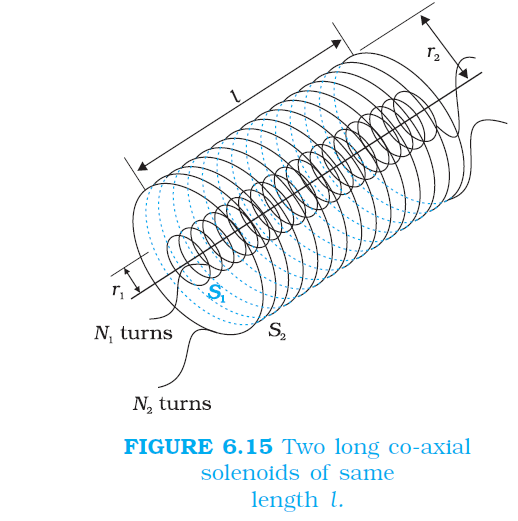
`color{blue} ✍️`Consider Fig. 6.15 which shows two long co-axial solenoids each of length l. We denote the radius of the inner solenoid `S_1` by `r_1` and the number of turns per unit length by `n_1.` The corresponding quantities for the outer solenoid `S_2` are `r_2` and `n_2`, respectively. Let `N_1` and `N_2` be the total number of turns of coils `S_1` and `S_2`, respectively.

`color{blue} ✍️`When a current `I_2` is set up through `S_2`, it in turn sets up a magnetic flux through `S_1`. Let us denote it by Φ1. The corresponding flux linkage with solenoid `S_1` is

`color{purple}(N_1Φ_1 = M_(12)I_2)` ..................(6.9)

`color {blue}{➢ ➢}` `M_(12)` is called the mutual inductance of solenoid `S_1` with respect to solenoid `S_2`. It is also referred to as the coefficient of mutual induction. For these simple co-axial solenoids it is possible to calculate `M_(12)`. The magnetic field due to the current `I_2` in `S_2 is μ_0n2_I_2.` The resulting flux linkage with coil `S_1` is,

`color{purple}(N_1 Φ_1 = (n_1l)(pir_(1)^(2)) (mu_0n_2I_2))`

`color{purple}(=mu_0 n_1n_2pir_(1)^(2)lI_2)` ...............(6.10)

`color {blue}{➢ ➢}` where `n_1l` is the total number of turns in solenoid `S_1`. Thus, from Eq. (6.9) and Eq. (6.10),

`color{purple}(M_(12)= mu_0 n_1n_2pir_(1)^(2)l)` .............6.11

`color{brown} bbul{"Note that"}` we neglected the edge effects and considered the magnetic field `color{purple}(μ0n_2I_2)` to be uniform throughout the length and width of the solenoid `S_2`. This is a good approximation keeping in mind that the solenoid is long, implying `l > > r_2`. We now consider the reverse case. A current `I_1` is passed through the solenoid `S_1` and the flux linkage with coil `S_2` is,

`color{purple}(N_2Φ_2 = M_(21) I_1)` ................(6.12)

`color {blue}{➢ ➢}` `M_(21)` is called the mutual inductance of solenoid `S_2` with respect to solenoid `S_1`. The flux due to the current `I_1` in `S_1` can be assumed to be confined solely inside `S_1` since the solenoids are very long. Thus, flux linkage with solenoid `S_2` is

`color{purple}(N_2Φ_2 = (n_2l)(pir_(1)^(2)) (mu_0n_2I_2))`

`color {blue}{➢ ➢}` where `n_2l` is the total number of turns of `S_2`. From Eq. (6.12),

`color{purple}(M_(21) = μ_0n_1n_2πr_1^2 l)` ............(6.13)

`color {blue}{➢ ➢}` Using Eq. (6.11) and Eq. (6.12), we get

`color{purple}(M_(12) = M_(21)= M)` (say) ...............(6.14)

`color{blue} ✍️`We have demonstrated this equality for long co-axial solenoids. However, the relation is far more general. Note that if the inner solenoid was much shorter than (and placed well inside) the outer solenoid, then we could still have calculated the flux linkage `N_1Φ_1` because the inner solenoid is effectively immersed in a uniform magnetic field due to the outer solenoid.

`color{blue} ✍️`In this case, the calculation of `M_(12)` would be easy. However, it would be extremely difficult to calculate the flux linkage with the outer solenoid as the magnetic field due to the inner solenoid would vary across the length as well as cross section of the outer solenoid.

`color {blue}{➢ ➢}` Therefore, the calculation of `M_(21)` would also be extremely difficult in this case. The equality `M_(12)=M_(21)` is very useful in such situations.

`color{blue} ✍️`We explained the above example with air as the medium within the solenoids. Instead, if a medium of relative permeability `μ_r` had been present, the mutual inductance would be

`color{purple}(M =μ_r μ_0 n_1n_2π r_(1)^(2) l)`

`color{blue} ✍️`It is also important to know that the mutual inductance of a pair of coils, solenoids, etc., depends on their separation as well as their relative orientation.

`color{blue} ✍️`Now, let us recollect Experiment 6.3 in Section 6.2. In that experiment, emf is induced in coil `C_1` wherever there was any change in current through coil `C_2`. Let Φ1 be the flux through coil `C_1` (say of `N_1` turns) when current in coil `C_2` is `I_2`.
Then, from Eq. (6.9), we have

`color{purple}(N_1Φ_1 = MI_2)`

`color {blue}{➢ ➢}` For currents varrying with time,

`color{purple}(d(N_1Φ_1)/(dt) = (d(MI_2))/(dt))`

`color {blue}{➢ ➢}` Since induced emf in coil `C_1` is given by

`color{purple}(epsilon_1 = (d(N_1Φ_1))/(dt))`

`color {blue}{➢ ➢}` We get,

`color{purple}(epsilon_1 = - M (dI_2)/(dt))`

`color{blue} ✍️`It shows that varying current in a coil can induce emf in a neighbouring coil. The magnitude of the induced emf depends upon the rate of change of current and mutual inductance of the two coils.

`color{blue} ✍️`In the previous sub-section, we considered the flux in one solenoid due to the current in the other. It is also possible that emf is induced in a single isolated coil due to change of flux through the coil by means of varying the current through the same coil. This phenomenon is called self-induction.

In this case, flux linkage through a coil of `N` turns is proportional to the current through the coil and is expressed as

`color{purple}(NΦ_B ∝ I)`

`color{purple}(NΦ_B = LI)` ..............(6.15)

where constant of proportionality L is called self-inductance of the coil. It is also called the coefficient of self-induction of the coil. When the current is varied, the flux linked with the coil also changes and an emf is induced in the coil. Using Eq. (6.15), the induced emf is given

`color{purple}(ε= - (d(NΦ_B))/(dt))`

`color{purple}(ε= -L(dI)/(dt))` .................(6.16)


Thus, the self-induced emf always opposes any change (increase or decrease) of current in the coil.

`color{blue} ✍️`It is possible to calculate the self-inductance for circuits with simple geometries. Let us calculate the self-inductance of a long solenoid of crosssectional area A and length l, having n turns per unit length. The magnetic field due to a current I flowing in the solenoid is `color{purple}(B = μ_0 n I)` (neglecting edge effects, as before). The total flux linked with the solenoid

`color{purple}(NΦ = (nl) (μ_0nI)(A))`

`color{purple}(= mu_0 n^2AlI)`

where nl is the total number of turns. Thus, the self-inductance is,

`color{purple}(L = (NΦ_B)/(I))`

`color{purple}(= μ n^2 Al)` ...............(6.17)

`color{blue} ✍️`If we fill the inside of the solenoid with a material of relative permeability `μ_r` (for example soft iron, which has a high value of relative permiability), then,

`color{purple}(L = μ_r μ_0 n^2 Al)` ...............(6.18)

`color{blue} ✍️`The self-inductance of the coil depends on its geometry and on the permeability of the medium. The self-induced emf is also called the back emf as it opposes any change in the current in a circuit. Physically, the self-inductance plays the role of inertia.

`color{blue} ✍️` It is the electromagnetic analogue of mass in mechanics. So, work needs to be done against the back emf `(ε )` in establishing the current. This work done is stored as magnetic potential energy. For the current I at an instant in a circuit, the rate of work done is

`color{purple}((dW)/(dt) = |epsilon|I)`

`color {blue}{➢ ➢}` If we ignore the resistive losses and consider only inductive effect, then using Eq. (6.16),

`color{purple}((dW)/(dt) = L I (dI)/(dt))`

`color {blue}{➢ ➢}` If we ignore the resistive losses and consider only inductive effect, then using Eq. (6.16),

`color{purple}((dW)/(dt) = L I (dI)/(dt))`

`color {blue}{➢ ➢}` Total amount of work done in establishing the current I is

`color{purple}(W = int dW = int_(0)^(I) LIdI)`

`color {blue}{➢ ➢}` Thus, the energy required to build up the current I is,

`W = 1/2 LI^2` ..................(6.19)

`color{blue} ✍️`This expression reminds us of `color{purple}(mv^2//2)` for the (mechanical) kinetic energy of a particle of mass m, and shows that L is analogus to m (i.e., L is electrical inertia and opposes growth and decay of current in the circuit).

`color{blue} ✍️`Consider the general case of currents flowing simultaneously in two nearby coils. The flux linked with one coil will be the sum of two fluxes which exist independently. Equation (6.9) would be modified into

`color{purple}(N_1 Φ_1 = M_(11)I_1 + M_(12) I_2)`

`color {blue}{➢ ➢}` where `M_(11)` represents inductance due to the same coil. Therefore, using Faraday’s law,

`color{purple}(epsilon_1 = - M_(11) (dI_1)/(dt) -M_(12) (dI_2)/(dt))`

`color {blue}{➢ ➢}` `M_(11)` is the self-inductance and is written as `L_1.` Therefore,

`color{purple}(epsilon_1 = - L_1(dI_1)/(dt) -M_(12) (dI_2)/(dt))`

`color{blue} ✍️`The phenomenon of electromagnetic induction has been technologically exploited in many ways. An exceptionally important application is the generation of alternating currents (ac).

`color{blue} ✍️`The modern ac generator with a typical output capacity of 100 MW is a highly evolved machine. In this section, we shall describe the basic principles behind this machine.

`color{blue} ✍️`The Yugoslav inventor Nicola Tesla is credited with the development of the machine.
As was pointed out in Section 6.3, one method to induce an emf or current in a loop is through a change in the loop’s orientation or a change in its effective area.

`color{blue} ✍️`As the coil rotates in a magnetic field B, the effective area of the loop (the face perpendicular to the field) is A cos θ, where θ is the angle between A and B. This method of producing a flux change is the principle of operation of a simple ac generator. An ac generator converts mechanical energy into electrical energy.

`color {blue}{➢ ➢}` The basic elements of an ac generator are shown in Fig. 6.16.



`color{blue} ✍️`It consists of a coil mounted on a rotor shaft. The axis of rotation of the coil is perpendicular to the direction of the magnetic field.

`color{blue} ✍️`The coil (called armature) is mechanically rotated in the uniform magnetic field by some external means.
The rotation of the coil causes the magnetic flux through it to change, so an emf is induced in the coil. The ends of the coil are connected to an external circuit by means of slip rings and brushes.

`color{blue} ✍️`When the coil is rotated with a constant angular speed ω, the angle θ between the magnetic field vector B and the area vector A of the coil at any instant t is `θ = ωt` (assuming `θ = 0º` at `t = 0`). As a result, the effective area of the coil exposed to the magnetic field lines changes with time, and from Eq. (6.1), the flux at any time t is

`color{purple}(Φ_B = BA cos θ = BA cos ωt)`

`color {blue}{➢ ➢}` From Faraday’s law, the induced emf for the rotating coil of N turns is then,

`color{purple}(ε= - N(dΦ_B)/(dt) = - MBAd/(dt) (cosomegat))`

`color {blue}{➢ ➢}` Thus, the instantaneous value of the emf is

`color{purple}(ε = NBAω sinωt)` ................(6.21)

`color {blue}{➢ ➢}` where `NBAω` is the maximum value of the emf, which occurs when `sin ωt = ±1.` If we denote NBAω as ε0, then

`color{purple}(ε = ε_0 sin ωt)` ...........(6.22)

`color {blue}{➢ ➢}` Since the value of the sine fuction varies between `+1` and `–1,` the sign, or polarity of the emf changes with time.

`color{brown} bbul{"Note"}` from Fig. 6.17 that the emf has its extremum value when `θ = 90º` or `θ = 270º,` as the change of flux is greatest at these points.

`color{blue} ✍️`The direction of the current changes periodically and therefore the current is called alternating current (ac). Since `ω = 2πν,` Eq (6.22) can be written as

`color{purple}(ε = ε_0sin 2π ν t)` ......................(6.23)

`color {blue}{➢ ➢}` where `ν` is the frequency of revolution of the generator’s coil. Note that Eq. (6.22) and (6.23) give the instantaneous value of the emf and ε varies between `+ε_0` and `–ε_0` periodically. We shall learn how to determine the time-averaged value for the alternating voltage.



`color{blue} ✍️`In commercial generators, the mechanical energy required for rotation of the armature is provided by water falling from a height, for example, from dams. These are called hydro-electric generators.

`color{blue} ✍️`Alternatively, water is heated to produce steam using coal or other sources. The steam at high pressure produces the rotation of the armature. These are called thermal generators. Instead of coal, if a nuclear fuel is used, we get nuclear power generators.

`color{blue} ✍️`Modern day generators produce electric power as high as `500` MW, i.e., one can light up `5` million `100` W bulbs! In most generators, the coils are held stationary and it is the electromagnets which are rotated. The frequency of rotation is `50` Hz in India. In certain countries such as USA, it is `60` Hz.