Mathematics LIMITS AND DERIVATIVES

LImit :

1. Concept Of Limits :


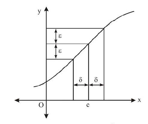
Suppose `f(x)` is a real -valued function `c` is a real number. The expression `lim_(x->c)f(x) = L` means that `f(x)` can be as close to `L` as desired by making `x` sufficiently close to `c`. In such a case, we say that limit of `f`, as `x` approaches `c`, is `L`. Note that this statement is true even if `f(c) ne L`. Indeed, the function `f(x)` need not even be defined at `c`. Two examples help illustrate this.

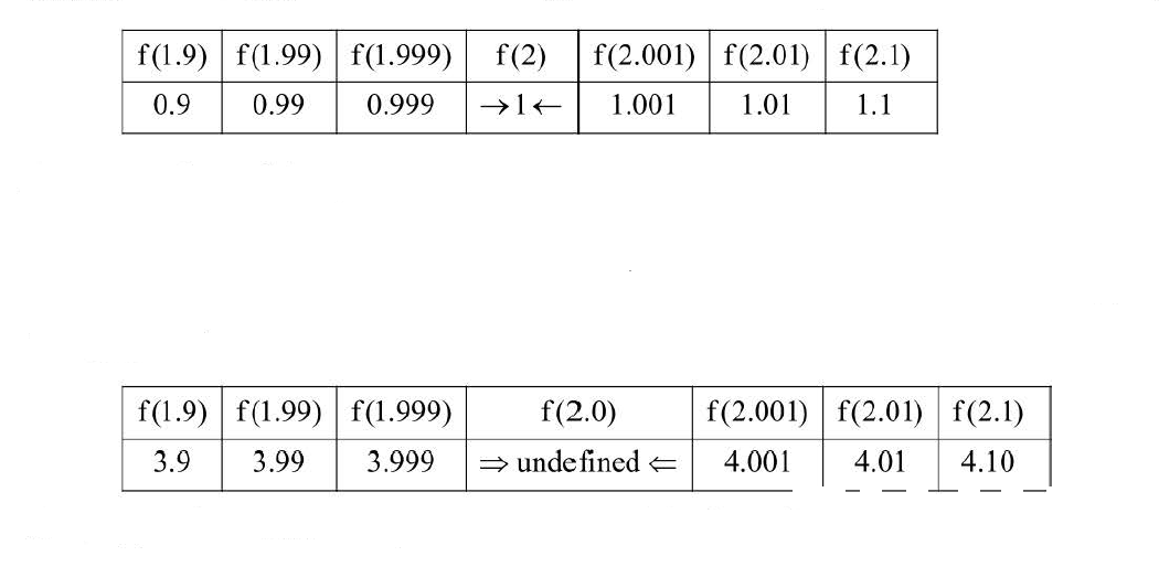
Consider `f(x) = x - 1` as `x` approaches 2. In this case, `f(x)` is defined at `2`, and it equals its limiting value `1`.


As `x` approaches `2`, `f(x)` approaches `1` and hence we have `lim_(x->2)f(x) =1`

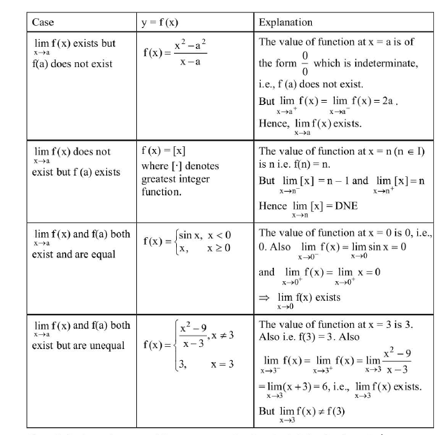
`f(x) =(x^2-4)/(x-2)` tn this case `x` approaches `2` the limiting value of `f(x)` is equal to `4` even if `f(x)` is not defined at `x = 2`.

Thus, `f(x)` can be made arbitrarily close to the limit of `4` just by making `x` sufficiently close to `2`.

Formal Definition of Limit :

Given for the sake of completeness but not used in exams.

Karl Weierstrass formally defined limit as follows :
Let `f` be a function defined on an open interval containing `c` (except possibly at `c`) and let `L` be a
real number.


`lim_(x->c) f(x) =L` means that for each real `epsilon > 0` there exists a real `delta > 0`
such that for all `x` with `0 < |x -c| < delta`, we have `|f(x) -L | < epsilon` or, symbolically.

` AA epsilon > 0, EE delta > 0, AA x ( 0< |x-c | < delta => |f(x) -L | < epsilon)`

Neighbourhood (NBD) of a point :

Let ` 'a' ` be a real number and let be a positive real number. Then the set of all real numbers lying between
`a-delta` and `a + delta` is called the neighbourhood of ` 'a' ` of radius ` 'delta' ` and is denoted by `N_delta (a)`.
Thus, `N_delta (a) = (a- delta, a + delta ) = {x in R | a - delta < x < a + delta}`
The set `(a - delta, a)` is called the left `NBD` of ` 'a'` and the set `(a, a + delta)` is known as the right `NBD` of `'a'`.


Left-and Right-Hand Limits :

Let `f(x)` be a function with domain `D` and let `'a'` be a point such that evety `NBD` of `a` contains infinitely
many points of `D`. A real number `l` is called left limit of `f(x)` at `x = a` iff for every `epsilon > 0` then exists a
`delta > 0` such that `a - delta < x < a =>` `| f(x) -l | < epsilon`.

In such a case, we write `lim_(x->a^-)f(x) =l`

Thus , `lim_(x->a^-)f(x) = l` , if `f(x)` tends to `l` as `x` tends to `'a'` from the left-hand side.

Similarly, a real number `l'` is a tight limit of `f(x)` at `x =a` iff for every `epsilon > 0`, there exists `delta > 0` such that
` a < x < a + delta => | f(x) - l | < epsilon` and we write `lim_(x->a^+) f(x) = l' `.

In order words, `I'` is a right limit of `f (x)` at `x = a` iff `f(x)` tends to `l'` as `x` tends to ` 'a' ` from the right-hand
side

Existence of Limit :

If follows from the discussions made in the previous two sections that `lim_(x->a) f(x) ` exist if `lim_(x->a^-) f(x) ` and
`lim_(x->a^+)f(x) ` exists and both are equal.

Thus `lim_(x->a) f(x) ` exist `<=> lim_(x ->a^-) f(x)= lim_(x->a^+)f(x).`

`f(a^-) = lim_(h->0) f (a-h)`
`f(a^+) = lim_(h->0) f(a+h)`

`lim_(x->a) f(x) ` exists `<=> f(a^-) = f (a^+)`

One sided limit :

Let the function `f(x)` is defined in `x in [a, b]`. Sometime we need to calculate `lim_(x->b)f(x) ` or `lim_(x->a)f(x)`. In such

`lim_(x->a) f(x) = lim_(x->a^+)f(x) =RHL` at `x=a`, as their is no left neighbourhood of `x =a`.

Similarly `lim_(x->b)f(x) = lim_(x->b^-)f(x) = LHL` at `x=b` . As their is no right neighbourhood of `x = b`.
for example , `f(x) = cos^(-1)x`

`lim_(x->1) f(x) = lim_(x->1^-)cos^-1 x=0`

`lim_(x-> -1) f(x) = lim_(x ->1^+) cos^-1 x =pi`


Difference between limit of function at `x = a` and `f (a)`:

Thus, for limit to exist at `x = a`, it is not necessary that function is defined at that point.

Sandwich Theorem Or Squeeze Play Theorem For Evalutating Limits :

`text(General:)` The squeeze principle is used on limit problems where the usual algebraic methods (factorisation
or algebraic manipulation etc.) are not effective. However it requires to "squeeze" our problem
in between two other simpler function whose limits can be easily computed and equal. Use of
Squeeze principle requires accurate analysis, in depth algebra skills and careful use of inequalities.

`text(Statement:)`

If `f`, `g` and `h` are `3` functions such that `f(x) le g (x) le h (x)` for all `x` in some interval containing the
point `x =c`, and if


`Lim_(x->c) f(x) = Lim_(x->c) h(x) = L => Lim_(x->c)g(x) =L`

From the figure note that `Lim_(x-> 0) g(x) =1`


Note: (i) the quantity `c` may be a finite number, `+ oo` or `-oo`.
Similarly `L` may be finite number, `+oo` or `-oo`.

Evaluation Of Trigonometric Limits :

`Lim_(theta -> 0) (sin theta)/theta=1` (where `theta` is in radians)

Proof: Consider a circle of radius r. Let `O` be the centre of the circle
such that `angleAOB = theta` where `theta` is measured in radians and it is very small.
Suppose the tangent at `A` meets `OB` produced at `P`. From figure, we
have


Area of `DeltaOAB <` Area of sector `OAB < ` Area of `Delta OAP`

`=> 1/2 OA xx OBsin theta < 1/2 (OA)^2 theta < 1/2 OA xx AP`

`=>1/2 r^2 sin theta <1/2 r^2 theta <1/2 r^2 tan theta` [ In `Delta OAP, AP = OA tan theta`]

`=> sin theta < theta < tan theta => 1> (sin theta)/theta > cos theta`

`=> 1> lim_(theta->0) (sin theta)/theta > lim_(theta->0) cos theta ` or `lim_(theta->0) cos theta < lim_(theta->0) (sin theta)/theta <1`

`=> 1 < lim_(theta->0) (sin theta)/theta <1 => lim_(theta->0) (sin theta)/theta =1` (By Sandwich Theorem)


`(ii)` `Lim_(theta->0) (sin theta)/theta =1`

We have `lim_(theta->0) (tan theta)/theta = lim_(theta->0)((sin theta)/theta ) (1/cos theta) = lim_(theta->0) ( (sin theta)/theta)*lim_(theta->0) (1/(cos theta)) =1`


`(iii)` `lim_(theta->a) (sin (theta-a))/(theta-a) =1`

We have `lim_(theta->a) (sin (theta-a))/(theta-a) = lim_(h->0) (sin(a+h-a))/(a+h-a)= lim_(h->0 )(sin h)/h =1`

`(iv)` `lim_(theta ->a) (tan (theta-a))/(theta-a)=1`


`(v) ` `lim_(theta->0) (sin^(-1) x)/x=1`

`(vi)` `lim_(x->0) (tan^(-1) x)/x=1`

`(vii)` `Lim_(x->oo) (1-cos x)/x^2 =1/2` (remember).


Note : Let `[.]` denotes greatest integer function

(i) `Lim_(x->0) [ sinx/x]=0` (ii) ` [ Lim_(x->0) (sinx)/x ]=1`

(iii) `Lim_(x->0) [ (tanx)/x] =1` (iv) `Lim_(x->0) [ (sin^-1) /x]=1`

(v) ` [Lim_(x->0) (sin^(-1 ) x)/x ]=0`


Indeterminate forms :

lndeterminant forms are `0/0 , oo/oo, oo -oo, 0 xx oo , 1^ oo ,0^0` and `oo^0`

Evaluation Of Algebraic Limits :
(i) Direct Substitution Method :

Consider the following limits : (i) `lim_(x->a)f(x)` (ii) `lim_(x->a) (phi (x))/(psi (x))`

If `f(a) ` and `(phi (a)) /(psi (a))` exist and are fixed real numbers and ` psi (a) ne 0` then we say that `lim_(x->a) f(x) = f(a)` and `lim_(x-a)(phi (x))/(psi(x)) = (phi (a)) /(psi (a))`

(ii) Fractorization Method :
Consider `lim_(x->a) (f(x))/(g(x))`

lf by substituting `x =a`, `f(x) /g(x) ` reduces to the form `0/0`, then `(x - a)` is a factor of both `f(x)` and `g(x)`. So,

we first factorize `f(x)` and `g(x)` and then cancel out the common factor to evaluate the limit.

(iii) Rationalization Method :
This is particularly used when either the numerator or the denominator or both involve expression consists

of squares roots and on substituting the value of `x` the rational expression takes the form `0/0, oo/oo`.
Following examples illustrate the procedure.

(iv) Evalutation of Algebraic Limit Using Some Standard Limits :
Recall the binomial expansion for any rational power
`(1+x)^n =1 +nx + (n(n-1)) /(2!) x^2 + (n(n-1) (n-2)) /(3!) x^3..........`
where `|x| <1`

When `x` is infinitely small (approaching to zero) such that we can ignore higher powers of x, then we have
`(1 + x)^n = 1 + nx` (approximately).

(v) Evaluation of Algebraic Limits at Infinity
We know that `lim_(x-> +oo) 1/x =0` and `lim_(x->+oo) 1/x^2=0`

`:.` `lim_(x->oo)f(x) = lim_(y-> 0)f (1/y)`

 
SiteLock