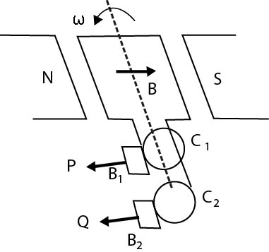
The Armature coil which is a rectangular coil of N turns
wound over a soft-iron core (to increase the
magnetization) is mounted on an axle along the
symmetry axis of the coiI that can be coupled to a
rotating wheel/turbine etc. A strong uniform magnetic
field produced by a permanent magnet or electromagnet
cuts through the rotating Armature coil as shown in the
figure. Notice that the axis of rotation for the Armature
coil is perpendicular to the magnetic field lines.

The Armature coil is also connected to two slip rings `C_1`
and `C_2` which in turn are in contact with two carbon brushes `B_1` and `B_2` such
that there is permanent electrical contact without hampering the
rotation of the coil . The brushes are connected to two
terminals P and Q which function as the output terminals
for the Generator and the external circuit is connected
across P and Q.

The armature coil is driven at a constant angular speed `omega`
such that at given instant, the angle between the coil's
area vector `vecA `and the magnetic field `vecB` is `theta = (omega t +phi)`,
therefore the magnetic flux, `phi_B=vecB.vecA` is given by the
relation.

`phi_B = NBACos(omega t+ phi)` . Hence, by application of Faraday's
law, the induced EMF (developed across the terminals P
and Q),

`E = - (dphi_B)/(dt) =NBA omega sin(omega t+phi)` which can be expressed as,
`E = E_0 sin (omega t +phi)` , where the term `E_0` is define as the
'peak' voltage given by `E_0 = NBA omega = NBA xx 2 pi f`.

It is important to note here that the peak voltage `E_0`
depends on not only the intensity of the magnetic field B,
the geometry of the Armature coil (N and A) but also on
the angular frequency `omega` (or frequency f) of rotation.

Household power supplied in India and most of
Asia/Europe is AC with an alternating frequency of 50 Hz.

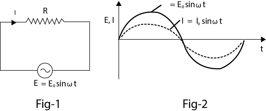
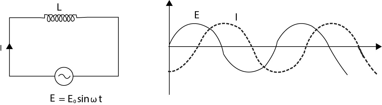
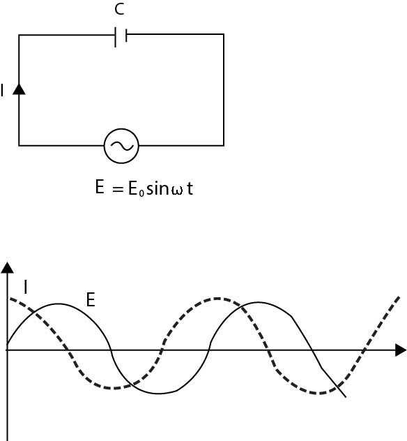
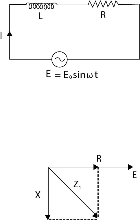
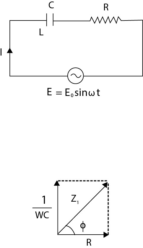
In the sections following, various types of circuits using
resistors, capacitors and inductors connected across an
AC Source are analyzed

For a circuit consisting of an alternating source
`E = E_0 sin(omega t)` with it's terminals connected across a
resistance `R` as shown in the diagram below, the
instantaneous current, Power etc can be derived as
follows. Such a type of a circuit is known as a "purely
resistive " AC circuit or simply a resistive circuit.(figure-1)

If the instantaneous current at some time `t=t` after the
switch was closed at `t=0` is `i` , by application of
Kirchhoff's loop law to the given circuit,

`E - iR = 0 => i= E/R= E_0/R sin (omega t)` which can be simply
denoted as
`i= i_0 sin(omega t)` where `i_0 =E_0/R` can be interpreted as the
'peak' current (or the maximum value of the
instantaneous current passing through the resistor).

Careful comparison of the expressions for instantaneous
current and voltage in the circuit leads to the important
conclusion that both `E` and `i` vary Sinusoidally with the
same angular frequency w and with identical phase. The
following figure represents the variation of current and
voltage super-imposed.

For an inductor `L` connected across the terminals of an
AC voltage source `E = E_0 sin(omega t) ` . the circuit is as shown
in the following figure-1. Note here that we assume that the
resistance of the connecting wires is a negligible
quantity. Such a circuit is called a purely inductive AC
circuit or simply an inductive circuit.
The induced emf across the inductor will be

`V_L =-L((di)/(dt))` where i is the instantaneous current passing
through it.

From application of Kirchhoff's loop law,

`E-L((di)/(dt)) =0`

`=> E_0 sin (omega t) -L((di)/(dt)) =0`

`=> int_i^tdi =E_0/L int_0^t sin (omega t) dt` where i' is the value of the

instantaneous current initially.

`i = i^' +E_0/L [(-cos (omega t)/omega)]_0^t`

`i = -(E_0/(omega L)) cos (omega t) + K`

where is K is some constant depending on the values of
constants `i^' L, omega` etc.

Now, it is understood that the voltage source of the circuit
being 'alternating' in nature, the current in the circuit must
be an 'alternating' current ( d.c . component of current
must be zero), hence the value of the constant K is taken
to be zero.

`=> -(E_0/(omega L) cos (omega t))` which can be expressed as

`=> i = i_0 sin(omega t - pi/2),` where peak current `i_0 = (E_0/(omega L))`

Therefore it is evident in the case of an inductive circuit,
the current 'lags' behind the voltage by a phase of `pi/2`
This can be further understood from the following graph
representing a superposition of current and voltage
variation with respect to time.(figure-2)

As seen in the above expression, the value of peak
current `i_0` is given by
`i_0 = (E_0)/(omega L)`
In this, the term `omega L` is defined as the 'inductive reactance
denoted as `X_L` , `X_L = omega L = 2 pi f L`

As the reactance `X_L` has the dimensions of electrical
resistance and represents the ratio of peak Voltage to
peak current `i_0 = (E_0/X_L)` it's value effectively represents
how much the inductor 'opposes' the flow of current
through it in such a circuit. It is interesting to note here
that `X_L` . is directly proportional to frequency f of the
alternating source, hence for an extreme case `f = 0` ( d.c
source), `X_L =0` , which agrees with the role of an inductor
in a de inductive circuit (L- R growth or decay circuits) at
steady state (it acts like a 'short circuit)

For a capacitor connected across the terminals of an AC
voltage source `E = E_0sin(omega t)` as shown in the following
figure-1. Such a circuit is called a purely capacitive AC
Circuit or simply capacitive circuit and again the
resistance of the connecting wires is assumed to be
negligible.

Now, let at time `t = t` , the current through the circuit is `i`
and the charge accumulated by the capacitor is q, the
voltage across the plates of the capacitor, `V_c= q/C` and

`i = + (dq)/(dt)` (see polarities in the diagram expressed for the

'positive' half cycle, in the negative half cycle simply
reverse all the polarities!)
Therefore, by application of Kirchhoff's loop law,

`E-V_c =0`

`=> E_0 sin (omega t) -q/c = 0`
`q = CE_0sin(omegat)`
Therefore, instantaneous current can be expressed as
`i=i_0sin(omega t + pi/2)`, where peak current `i_0 = (omega C E_0) = E_0/X_c`
`X_c` being the capacitive reactance, it can be shown that
`X_c = 1/(omega C) =1/(2 pi f C), ` `X_c` has dimensions of resistance and
can be interpreted as the effective resistance offered by
the capacitor in this type of circuits. Note that capacitive
reactance is inversely proportionate to the frequency of
the source and hence for a d.c circuit (f=0), the capacitor
effectively 'blocks' current.

Also, the current in a purely capacitive circuit "leads"
ahead of the voltage by a phase of `pi/2` This can be further
understood from the following graph representing a
superposition of current and voltage variation with
respect to time.

As is evident from the sections above, currents and
voltages in AC circuits are quantities that vary with time
sinusoidally and therefore have 'phase'. Therefore in
dealing with mathematical operations involving these
quantities, the phase difference between two alternating
physical quantities becomes important and an effective
way to deal with this is the phasor analysis method.
In this method, sinusoidally varying quantities are
represented geometrically as 'phasors' (similar to the
geometrical representation of vectors) and while adding
such quantities. the phase difference is used to determine
the resultant (similar to the case of vector addition)

In a phasor diagram, the phase for the voltage is taken to
be zero, the phase for current is then represented
according to the phase difference (the 'lag' or 'lead') for
the current with respect to the voltage.

In this particular circuit the
voltage is in phase with the current. Hence, there is no
phase lag between the two, hence it can be represented
by a simple phasor diagram shown below

In this particular circuit the
current leads the voltage by phase angle of `pi/2`. Hence,
the phasor diagram can be represented as in the figure.

In this particular circuit the
current lags the voltage by phase angle of `pi/2` Hence, the
phasor diagram can be represented as in the figure


Now, based upon the phasor analysis method developed
above, the analysis of circuits with combinations of
resistors. inductors and capacitors connected across an
AC voltage source is as follows.

In this type of circuit an inductor of inductance `L` is
connected in series to a resistance `R` and the
combination is connected across the terminals of an `AC`
source `E = E_0 sin(omega t)`

Now in this particular circuit, the inductor will cause the
current to lag behind the voltage by some phase angle `phi`
however this will not be `pi/2` , due to the presence of the

resistor. The resistance `R` and the inductive reactance `X_L`
are combined by the phasor analysis method to
determine the impedance 'Z' of the circuit, where Z has
dimensions of resistance and is the ratio of peak voltage
and peak current `i_0 = E_0/Z`

From the phasor diagram

`Z= sqrt(R^2 +X_L^2) = sqrt(R^2 + (omega L)^2)`
And resultant phase angle by which the current lags
behind voltage is

`phi = tan^-1(X_L/R)`
The instantaneous current can therefore be expressed as
`i = i_0 sin (omega t - phi)` where `i_0 = E_0/Z` is the peak voltage.

In this type of circuit a capacitor `C` is connected in series
to a resistance `R` and the combination is connected
across the terminals of an `AC` voltage source
`E = E_0 sin (omega t)` as shown in the figure alongside.

In this particular circuit the Capacitor has a tendency to
make the current lead the voltage by a certain phase
angle `phi` , however this will not be `pi/2`, due to the presence

of the resistor. The resistance R and the capacitive
reactance `X_c` are combined by the phasor analysis
method to determine the impedance 'Z' of the circuit,
where `Z` has dimensions of resistance and is the ratio of
peak voltage and peak current `i_0 =E_0/Z` The phase
diagram below can be used to determine Z and `phi`

`Z =sqrt(R^2 +X_c^2) = sqrt(R^2 + (1/(omega C))^2)` and `phi =tan^-1(X_c/R)`

The instantaneous current can therefore be expressed as

`i= i_0 sin(omega t +phi)` where `i_0 = E_0/Z` is the peak voltage.

An LC circuit, also called a resonant circuit, tank circuit, or tuned circuit, is an electric circuit consisting of an inductor, represented by the letter L, and a capacitor, represented by the letter C, connected together. The circuit can act as an electrical resonator, an electrical analogue of a tuning fork, storing energy oscillating at the circuit's resonant frequency.

LC circuits are used either for generating signals at a particular frequency, or picking out a signal at a particular frequency from a more complex signal. They are key components in many electronic devices, particularly radio equipment, used in circuits such as oscillators, filters, tuners and frequency mixers.


`text(LC OSCILLATIONS :)`

Consider an LC circuit in which a capacitor is connected to an inductor, as shown in Figure.

Suppose the capacitor initially has charge `Q_0`. When the switch is closed, the capacitor begins to discharge and the electric energy is decreased. On the other hand, the current created from the discharging process generates magnetic energy which then gets stored in the inductor. In the absence of resistance, the total energy is transformed back and forth between the electric energy in the capacitor and the magnetic energy in the inductor. This phenomenon is called electromagnetic oscillation.

The total energy in the LC circuit at some instant after closing the switch is

`U=U_C + U_L= 1/2 Q^2/C +1/2 LI^2`

The fact that U remains constant implies that

`(dU)/(dt)=d/(dt)(1/2 Q^2/C + 1/2 LI^2)=Q/C (dQ)/(dt) + LI (dI)/(dt)=0`

`Q/C + L(d^2Q)/(dt^2)=0`

where `I=-(dQ)/(dt)`

and `(dI)/(dt)=-(d^2Q)/(dt^2)`

Notice the sign convention we have adopted here. The negative sign implies that the current I is equal to the rate of decrease of charge in the capacitor plate immediately after the switch has been closed.

The general solution to equation is

`Q=Q_0 cos (omega_0t+phi)`

where `Q_0` is the amplitude of the charge and `phi` is the phase. The angular frequency `omega_0` is given by

`omega_0 = 1/sqrt(LC)`

The corresponding current in the inductor is

`I=-(dQ)/(dt)=omega_0Q_0sin(omega_0t +phi)=I_0sin(omega_0t+phi)`

where `I_0=omega_0Q_0`

From the initial conditions `Q (at// t = 0) = Q_0` and `I (at //t = 0) = 0`, the phase `phi` can be determined to `phi = 0`. Thus, the solutions for the charge and the current in our LC circuit are

`Q(t)=Q_0cosomega_0t`

and `I(t)=I_0sinomega_0t`

The time dependence of `Q(t)` and `I(t)` are depicted in figure.

Using Eqs., we see that at any instant of time, the electric energy and the magnetic energies are given by

`U_E=(Q^2(t))/(2C)=((Q_0^2)/(2C))cos^2omega_0t`

and `U_B=1/2LI^2(t)=(LI_0^2)/2 sin^2omegat=(L-omega_0Q_0)^2/2 sin^2omega_0t=(Q_0^2/(2C))sin^2omega_0t`

The electric and magnetic energy oscillation is illustrated in figure.

The mechanical analog of the LC oscillations is the mass-spring system, shown in Figure.

If the mass is moving with a speed v and the spring having a spring constant k is displaced from its equilibrium by x, then the total energy of this mechanical system is

`U=K+U_(sp)=1/2mv^2+1/2kx^2`

where Kand `U_(sp)` are the kinetic energy of the mass and the potential energy of the spring, respectively.
In the absence of friction, U is conserved and we obtain

`(dU)/(dt)=d/(dt)(1/2mv^2+1/2kx^2)=mv(dv)/(dt)+kx(dx)/(dt)=0`

Using `v=(dx)/(dt)` and `(dv)/(dt)=(d^2x)/(dt^2)`

the above equation may be rewritten as

`m(d^2x)/(dt^2)+kx=0`

The general solution for the displacement is

`x=x_0cos(omega_0t+phi)`

where `omega_0=sqrt(k/m)`

is the angular frequency and `x_0` is the amplitude of the oscillations. Thus, at any instant in time, the energy of the system may be written as

`U=1/2 mx_0^2omega_0^2sin^2(omega_0t+phi)+1/2kx_0^2cos^2(omega_0y+phi)`

`=1/2kx_0^2[sin^2(omega_0t+phi)+cos^2(omega_0t+phi)]=1/2kx_0^2`

In figure we illustrate the energy oscillations in the LC circuit and the mass spring system (harmonic oscillator).