In this case, the motion of the particle (or body)
involved is to and fro along a straight line, besides
the other necessary conditions.

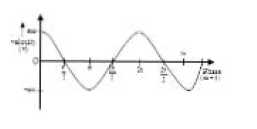
Let a particle `P` perform oscillatory motion between
two fixed points `A` and `B`. Let `O` be the mid point of
`A` and `B`. (fig.) If the particle `P` oscillates about point
`O` in such a way that its acceleration `f` , at any
position when its displacement from O is `x` , can be
mathematically expressed as `f` `x` and is directed
towards `O`, then its motion will be `SHM`. Here, the
point `O` is known as mean or stable or
equilibrium or neutral position, and in case of "simple"
harmonic motion , the maxim tun displacement, of
the particle on either side of the mean position is
the same i.e. `O A = OB` .


Now, taking the motion of the particle to be along Xaxis,
SHM can be mathematically expressed as

`vecf = (-omega^2)vecx...........................(1)`

Here, the negative sign stands for the fact that the
direction of acceleration is opposite to that of
displacement, and `omega^2` is a positive constant.

Again, if m be the mass of the oscillating particle (or
body), then, multiplying both sides of eqn. (1) by m,
we have

`mvecf = (-momega^2)vecx` or `vecF = (-k)vecx......................(2)`

where `mvecf = vecF` is the force acting on the particle and
k = `m omega^2` a positive constant.

Equations (1) or (2) can equally be used to show
that a given motion is SHM.

From equation (2) it is evident that `X = 0 ; F = 0`
which shows that the particle experiences no force,
when at mean position, it will not oscillate.
However, if it is disturbed even slightly by external
force, then new forces (restoring forces) should be
set up in the system which should tend to bring the
particle to its mean position. Depending upon the
nature of restoring forces, we have several types of
SHM. The restoring forces can be electrical,
gravitational, magnetic, elastic etc.

From equation (1),
`f = -omega^2 x` [Omitting the vector sign]
or `(dv)/(dt) =- omega^2 x`
`(dv)/(dx)*(dx)/(dt) = -omega^2x`
` => vdv = -omega^2x dx`

Integrating both sides, we get `v^2/2 = (- omega^2 x^2)/2 +C_1`

where `C_1` is a constant of integration. Since the
velocity of the particle is zero at its extreme
position `x = a` (say)

`0= (-omega^2 a^2)/2 +C_1`
`C_1 = (omega^2 a^2)/2`

Substituting for `C_1` we get

`v^2/2 = (-omega^2x^2)/2 + (omega^2x^2)/2` or `v^2 = omega^2(a^2-x^2)`

`v= + omega (a^2 -x^2)^(1/2)............................(3)`

Again,

`V = (dx)/(dt)`

From equation (3) `(dx)/(sqrt(a^2-x^2)) = omega dt`

Integrating both sides, we get

`sin^-1(x/a) = omega t +C_2`

Where `C_2` is a constant of integration; let at `t=0` ; `x=x_0`


Then, `sin^-1(x_0/a) = C_2 = f` (say)
Then the above equation can be rewritten as

`sin^-1(x/a) = omega t +f`

`x/a = sin (omega t +f)`

`x= a sin (omega t +f).................................(4)`

Rewriting equation (3), by substituting for `x` in
terms oft from (4), we have

`v= omegasqrt[a^2 -a^2sin^2(omega t +f)]`

`v= omega a cos (omega t +f).......................(5)`

Also, rewriting equation (1), by substituting for x in
terms oft from (4), we have

`f = -omega^2 a sin(omega t+f)..............................(6)`

Equations (1) and (3), express the acceleration and
velocity of a particle executing `S H M` in terms of
displacement.

Equation (4), (5) and (6) express displacement,
velocity and acceleration, in terms of time.

(a) Amplitude :
It is the maximum displacement of
the particle executing SHM from its mean position.
From equation (4), it is obvious that the
displacement varies between the limits `- a` to `+a` as
`sin( omega t + f)` varies continuously between the limits
`-1` and `+1` respectively.
Thus, amplitude `= | X_(max) | = a`

We have discussed earlier that all SHMs are periodic
motions which repeat themselves in equal time
intervals. This minimum time interval is known as
time period for the oscillations.

Let T be the time period for the oscillation, then
from equation (4), `x = a sin ( omega t + f) = a sin [ omega (t +
T) + f )`

`sin(omega t + f) = sin(omega t +f + omega T)`

Since all sine and cosine functions vary periodically
with an angle `2 p`

`omega T = 2p` `=> T=(2pi)/omega`

The number of revolutions (expressed in radian ) performed per
unit time is known as angular frequency.

(Each oscillation corresponds to one revolution; see
more in the next article)

In a time T (time period), no. of revolution covered
=1

In a time of 1 sec. no. of revolutions covered `= 1/T`
Angle described in each revolution `= 2 p`

Angle described in `1/T` revolution `=(2pi)/T`
Thus, angular frequency `= (2pi)/T =omega`
The number of oscillations described per unit time
is known as the frequency of oscillations.
Evidently, frequency `n = 1/T`

We have seen earlier, that the
displacement, velocity and acceleration of a particle
executing SHM vary periodically with the angle `( omega
t + f )` associated with the sine or cosine term.
Knowing this angle, we can be sure of its position as
well as state of motion as to how and where is it
oscillating. This angle `( omega t + f )` is known as the
"phase" of the oscillating particle . Since the phase
is a time dependent factor, it will be more
worthwhile to speak in terms of instantaneous
phase (i.e., phase at any instant).

Taking the displacement equation as `x = a sin ( omega t +
f)`

we have at `omega t + f = 0 ; x = 0`
at `omega t + f = p /2 ; x = a`
at `omega t + f = p ; x = 0`
at `omega t + f = 3 p /2 ; x = -a` and so on.
Notice that, as time varies indefinitely, phase keeps
on changing, between `0` to `2 p` ; the reason being `( omega
t + f) = ( omega t + f ) + 2 n p` where `n = I`.

The phase of a particle executing SHM, initially (i.e., at the instant
when time was reckoned) is known as the initial
phase or phase constant or epoch .

Since instantaneous phase `= omega t + f` , so

Initial phase can be obtained by putting `t = 0`
Phase constant `= f`

As a special case, If at the instant of start of motion phase be zero, then `f = 0`.
All, the equation can be rewritten by replacing `( omega t
+f)` with `omega t`.
Considering the displacement equation as
`x = a sin ( omega t + f )`
Let us put `f = (pi/2 + phi)` the displacement equation
becomes

`x = a sin (omega t + pi/2 +phi' )`

`= a cos(omega t +f^')`

Differentiating w.r.t. time `t`
`v =-a omega sin( omega t+f ')`
and `f = - a omega^2 cos ( omega t + f ')`
`= - omega^2x`

The above equation too represent various
parameters associated with SHM.

Let the phase of a particle at time `t_1` be `f_1` , then
`f_1 = omega t_1 + f ........ (a)`
Let the phase of the particle change to `f_2` , at time
`t_2`, then
`f_2 = omega t_2 + f ........ (b)`
Subtracting (a) from (b)
Phase difference `f_2 - f_1 = omega(t_2 - t_1)`

or `D f = omega D t`
Putting `D t = T` and `omega = (2pi)/T` , we have `D f = 2 p`

Thus, a phase difference of `2 p` is equivalent to a
time difference T.

Similarly, a phase' difference of p is equivalent to a
time difference of `T/2`, and so on.

Assuming the displacement equation to be `x = a sin
omega t` , clearly the graph will be a sine curve. (Figure)

Putting `x = 0`, we have `sin (omega t) = 0`
`omega t_n = n p` , where `t_n = npi/omega`
Putting `n = 0, 1, 2, 3` etc.
we get
`t_0 =0, t_1 =pi/omega, t_2 = (2pi)/omega , t_3 = (3 pi)/omega` etc.
and putting `x = +- a` (i.e., maximum displacement)
we get `sin ( omega t) = + 1`
`omega t_n = (2n + 1)(pi/2)` where `n = I`
Purring `n = 0, 1, 2` etc. we get
`t_0 = pi/(2omega), t_1 = (3pi)/(2omega), t_2 = (5pi)/(2omega)` etc.

Assuming `x =a sin omega t` , we get on differentiating `omega t = 0`
`v =a omega cos omega t`

Putting `v = 0`, we get `cos omega t = 0`
`omega t_n = (2n + 1)pi/2`
Putting `n = 1, 2` , etc.

`t_0 = pi/(2a) , t_1 = (3 pi)/(2a) , t_2 = (5 pi)/(2a) ` etc.

Putting `v = +- a omega` (velocity amplitude), we get

`cos omega t = +- 1`

`omega t_n = n p` where `n =I`

`t_n = (n pi)/omega` putting `n = 0, 1, 2` etc.
we get `t_0 = 0 , t_1 = pi/omega , t_2 = (2 pi)/omega` etc
The graph is a cosine curve (Figure)

Assuming `x = a sin omega t`,
we have `f= -omega^2 x = -w^2 a sin omega t`
Putting `f = 0` , the instants at which `f = 0` , can be
found.
`sin omega t =0` `omega t_n = n p`

Putting `n = 0, 1, 2, ...... t_0 = 0, t_1 = pi/omega , t_2 = (2pi)/omega` etc.
Putting `f = pmomega^2a` ;
we have `sin omega t = +- 1` (acceleration amplitude)
`omega t_n = +-(2n + 1) pi/2`
Putting `n = 0, 1, 2,` etc.
`t_0 = pi/(2omega) , t_1 = (3pi)/(2omega) t_2 = (5pi)/(2omega)` : etc.
dearly the graph is a sine curve (Figure)

Since acceleration `(f) = -omega^2 (x)` . The variation is
linear.

We have seen earlier that
`v = omega sqrt(a^2-x^2)`
`v^2 = w^2(a^2 -x^2)`
`v^2/omega^2 = a^2 , x^2 (x^2/a^2 +v^2/(a^2 omega^2)) =1`
The graph is an ellipse. (figure)

from the equation `x =a sin ( w t + f)`
`x = 0` at` ( w t + f ) = n p` where `n in I`
and `x = pm a ` at ` ( w t +f) = (2n + 1)pi/2` , where `n in I`
The graph is a sine curve .

From the equation `v = a w cos ( w t + f )`
`v = 0` at `( w t + f) = (2n +1)pi/2` . where `n in I` and
`v =+-a w` at `( w t + f) = n p` , where `n in I`
The graph is shown in figure