(a) Definition: The median is the score that divides the distribution into halves; half of the scores are above
the median and half are below it when the data are arranged in numerical order. The median is also
referred to as the score at the 50th percentile in the distribution.

(i) Individual series : If the data is raw, arrange in ascending or descending order. Let n be the number of
observations.

lf `n` is odd, Median = value of `( (n+1)/2)^(th)` item.

lf `n` is even, Median `=1/2 ` [ value of `( n/2)^(th)` item + value of `((n/2)+1)^(th)` item ].



(ii) Discrete series :


In this case, we first find the cumulative frequencies ofthe variable arranged in ascending
or descending order and the median is given by Median `= ((n/2 )+1)^(th)` observation, where n is the cumulative
frequency.

(iii) For grouped or continuous distributions : In this case, following formula can be used.

Medtan `= l +( ( (N/2) -C )/f ) xx i`




where `l =` Lower limit of the median class
`f =` Frequency of the median class
`N =` The sum of all frequencies
`i =` The width of the median class
`C =` The cumulative frequency of the class preceding to median class.

Quartile : As median, divides a distribution into two equal parts, similarly the quartiles, quantiles, deciles
and percentiles divide the distribution respectively into `4, 5, 10` and `100` equal parts. The `j^(th)` quartile is

given by `Q_j = l + ( ( j (N/10) -C )/f ) i`.

Mode is the most frequent score in the distribution. A distribution where a single score is most frequent
has one mode and is called unimodal. When there are ties for the most frequent score, the distribution is
bimodal if two scores tie or multimodal if more than two scores tie.
Mode for continuous series

Mode ` = l_1 + [ (f_1 -f_0) / (2f_1 -f_0 -f_2) ]xx i`

Where, `l_1 =` The lower limit of the model class
`f_1 =` The frequency of the model class
`f_0 =` The frequency of the class preceding the model class
`f_2 =` The frequency of the class succeeding the model class
`i =` The size of the model class.

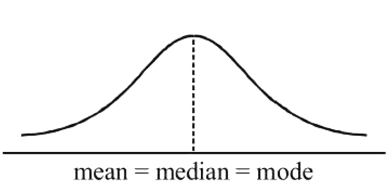
A distribution is a symmetric distribution if the values of mean, mode and median coincide. In a symmetric
distribution frequencies are symmetrically distributed on both sides of the centre point of the frequency
curve.


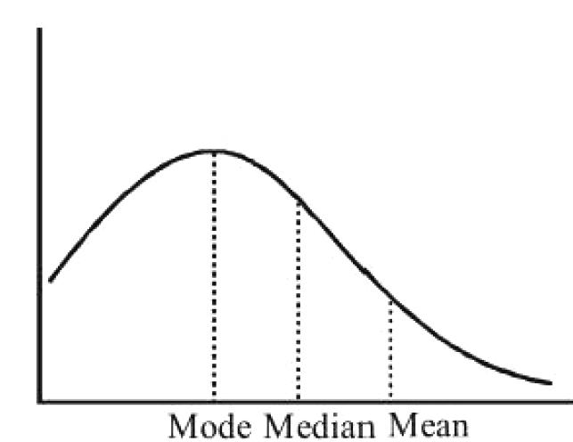
A distribution which is not symmetric is called a skewed distribution. ln a moderately asymmetric
distribution, the interval between the mean and the median is approximately one-third of the interval
between the mean and the mode i.e., when have the following empirical relation between them,


Mean - Mode `= 3` (Mean - Median) `=>` Mode `= 3` Median `- 2` Mean. it is known as Empirical relation.

A distribution is positively skewed when is has a tail extending out to the right (larger numbers) When a
distribution is positively skewed, the mean is greater than the median reflecting the fact that the mean is
sensitive to each score in the distribution and is subject to large shifts when the sample is small and
contains extreme scores.



Mean > Median > Mode

A negatively skewed distribution has an extended tail pointing to the left (smallernumbers) and reflects
bunching of numbers in the upper part of the distribution with fewer scores at the lower end of the
measurement scale.




Mean < Median < Mode.


In a moderately asymmetric distribution, the interval between the mean and the median is approximately
one-third of the interval between the mean and the mode i.e., when have the following empirical relation
between them,
Empirical formula: mode `= 3` median `- 2` mean

Coefficient of skewness `=` (Mean - Mode) ` / sigma `

Limitations of central values:
An average, such as the mean or the median only locates the centre of the data and does not tell us
anything about the spread of the data.

Measures of variability provide information about the degree to which individual scores are clustered
about or deviate from the average value in a di stribution i.e.,
The degree to which numerical data tend to spread about an average value is called the dispersion of the
data. The four measure of dispersion are

(i) Range (ii) Mean deviation

(iii) Variance (iv) Standard deviation



Important Note:

(a) A small value fora measure of dispersion indicate that the data are clustered closely (the mean is therefore
representative of the data).
(b) A large value of dispersion indicates that the mean is not re liable (it is not representative of the data).

The simplest measure of variability to compute and understand is the range. The range is the difference
between the highest and lowest score in a distribution. Because it is based solely on the most extreme
scores in the distribution and does not fully reflect the pattern of variation within a distribution, the range
is a very limited measure of variability.



Coefficient of range `: (L-S)/(L+S)`

`L =` Largest value
`S =` Smallest value

The arithmetic average of the deviations (a ll taking positive) from the mean, median or mode is known as
mean deviation.

(a) Mean deviation from ungrouped data (or individual series)

Mean deviation `= 1/N sum_(i =1)^(n) | x_i -M|`

Where `sum_(i=1)^n |x_i -M |` is the sum of modulus of the deviation of the variate from the mean (mean, median

or mode) and `N` is the number of terms.


(b) Mean deviation from continuous series :
Here first of all we find the mean from which deviation is to be taken. Then we find the deviation

`|x_i -M|` of each variate from the mean M and multiply these deviations by the corresponding frequency


So, Mean deviation `= 1/N sum_(i=1)^(n) f_i |x_i -M|`, where `N= sum _(i=1)^(n) f_i`.