Chemistry ELEMENTARY AND COMPLEX REACTIONS

Parallel Reactions :

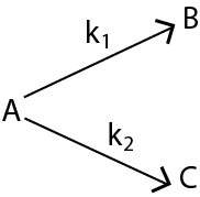
In such reactions (mostly organic) a single reactant gives two products `B` and `C` with different rate constants. If we assume that both
of them are first order, we get.

`-(d[A])/(dt)=k_1[A]+k_2[A]=k_1+k_2[A]`..........(1)

`(d[B])/(dt)=k_2[A]`..........(2)

And `(d[C])/(dt)=k_2[A]`.......(3)

Let us assume that in a time interval, `dt, x` moles/lit of `B` was produced and `y` moles/lit of `C` was produced.

`(d[B])/(dt)=x/(dt)` and `(d[C])/(dt)=v/(dt)` `((d[B])/(dt))/((d[C])/(dt))=x/y`.

We can also see that from (2) and (3), `((d[B])/(dt))/((d[C])/(dt)) =k_1/k_2`

`x/y=k_1/k_2` This means that irrespective of how much time is elapsed, the ratio of concentration of `B` to that of `C` from the start (assuming no `B` and `B` in the beginning) is a constant equal to `k_1//k_2`

Sequential Reactions :

`A overset(k_1)-> B overset(k_2)-> C`. In this `A` decomposes to `B` which in turn decomposes to `C`.

`(-d[A])/(dt)=k_1[A]`............(1)

`(d[B])/(dt)=k_1[A]-k_2[B]`..........(2)

`(d[C])/(dt)=k_2[B] ` ..............(3)

Integrating equation (1), we get `[A]=[A]_0 e^(-k_1 t)`

Now we shall integrate equation (2) and find the concentration of `B` related to time `t`.

`(d[B])/(dt)=k_1[A]-k_2[B]=> (d[B])/(dt)+k_2[B]=k_1[A]`

substituting `[A]` as `[A]_0 e^(-k_1t) => (d[B])/(dt)+k_2[B]=k_1[A]_0 e^(-k_1 t)` ........(4)

Integration of the above equation is not possible as we are not able to separate the two variables, `[B]` and `t`. Therefore we multiply equation (4) by an integrating factor `e^(k_2 t)` on both the sides of the equation.

`((d[B])/(dt)+k_2[B]) e^(k_2 t)=k_1 [A]_0 e^((k_2-k_1)t)`

We can see that the left hand side of the equation is a differential of `[B] e^(k_2 t)` .

`d/(dt) ([B] e^(k_2 t))=k_1[A]_0 e^((k_2-k_1)t) => d([B] e^(k_2 t))=k_1[A]_0 e^((k_2-k_1)t) dt`

Integrating within the limits `0` to `t`.

`int d ([B] e^(k_2 t)) =k_1[A]_0 int_0^t e^((k_2-k_1)t) => [B] e^(k_2 t)= k_1 [A]_0 [e^((k_2-k_1)t)/((k_2-k_1))]_0^t`

`=> [B] e^(k_2 t)= (k_1[A]_0)/(k_2-k_1) [e^((k_2-k_1)t)-1] `

`=> [B]=(k_1[A]_0)/(k_2-k_1) e^(-k_2t) [e^((k_2-k_1)t)-1]`

`[B]=(k_1[A]_0)/(k_2-k_1) [e^(-k_1 t)-e^(k_2 t)]` ........ (5)

Now in order to find [C], substitute equation (5) in equation (3), we get

`(d[C])/(dt)=(k_1k_2[A]_0)/(k_2-k_1) [e^(-k_1t)-e^(-k_2 t)]` `=> d[C]=(k_1k_2[A]_0)/(k_2-k_1) [e^(-k_1t)- e^(-k_2 t)] dt`

On integrating `int d[C]=(k_1k_2[A]_0)/((k_2-k_1)) int_0^t [e^(-k_1t) - e^(-k_2 t)] dt`

`=> [C]=(k_1k_2[A]_0)/((k_2-k_1)) [(e^(-k_1 t)/(-k_1))_0^t -(e^(-k_2 t)/(-k_2))_0^t]`

`=> [C]=(k_1k_2[A]_0)/((k_2-k_1)) [((e^(-k_1 t) -1)/(-k_1)) -((e^(-k_2 t) -1)/(-k_2))]`

`=> [C]=(k_1k_2[A]_0)/((k_2-k_1)) [(1-(e^(-k_1 t))/(k_1)) -((1-e^(-k_2 t))/(k_2))]`

`=> [C]=([A]_0)/(k_2-k_1) [k_2 (1-(e^(-k_1 t)) -k_1(1-e^(-k_2 t))]`

`B_text(max)` `text(and)` `t_text(max)` :

We can also attempt to find the time when `[B]` becomes maximum. For this we differentiate equation(5) and find `(d[B])/(dt)` & equate it to zero.

`(d[B])/(dt) = (k_1 [A]_0)/((k_2 -k_1)) [e^(-k_1t) (-k_1) + e^(-k_2t) (k_2)] = 0`

`=> k_1 e^(-k_1t) = k_2 e^(-k_2t) => k_1/k_2 = e^((k_1-k_2)t)`

Taking `log` of both the sides

therefore `t_(max) = 1/(k_1 -k_2) ln(k_1/k_2)` ..........(6)

Substituting equation (6) in equation (5)

`B_text(max) = [A]_0 [k_2/k_1]^((k_2)/(k_1 -k_2))`

 
SiteLock