POTENTIAL DUE TO AN ELECTRIC DIPOLE
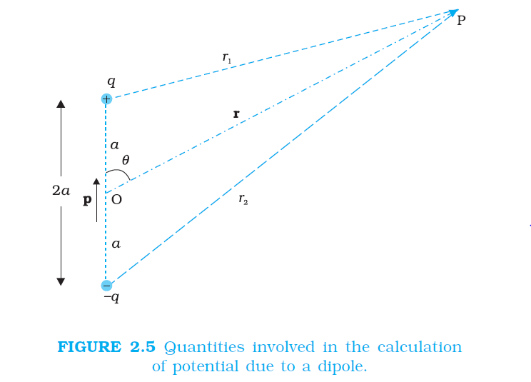
`color{blue} ✍️` As we learnt in the last chapter, an electric dipole consists of two charges `q` and `–q` separated by a (small) distance `2a.`
`color{blue} ✍️` Its total charge is zero. It is characterised by a dipole moment vector `p` whose magnitude is `q × 2a` and which points in the direction from `–q` to `q` (Fig. 2.5).
`color{blue} ✍️` We also saw that the electric field of a dipole at a point with position vector `r` depends not just on the magnitude `r,` but also on the angle between `r` and `p`.
`color{blue} ✍️` The field falls off, at large distance, not as `1/r^2` (typical of field due to a single charge) but as `1//r^3.`
`color{blue} ✍️` We, now, determine the electric potential due to a dipole and contrast it with the potential due to a single charge. As before, we take the origin at the centre of the dipole.
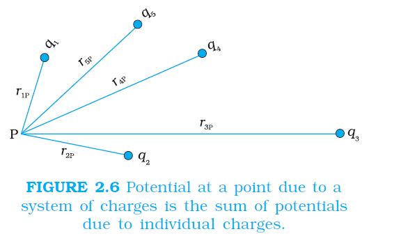
`color{blue} ✍️` Now we know that the electric field obeys the superposition principle. Since potential is related to the work done by the field, electrostatic potential also follows the superposition principle. Thus, the potential due to the dipole is the sum of potentials due to the charges `q` and `–q.`
`color{blue}(V = 1/(4piepsilon_0) (q/r_1-q/r_2))` .................2.9
`color{blue} ✍️` where `r_1` and `r_2` are the distances of the point P from q and –q, respectively.
Now, by geometry,
`color{purple}(r_(1)^(2) = r^2 + a^2 − 2ar cosθ)`
`color{purple}(r_(2)^(2) = r^2 + a^2 + 2ar cosθ)` ................2.10
`color{blue} ✍️` We take r much greater than a `(r >> a )` and retain terms only upto the first order in `a/r`
`color{blue} ✍️` We take r much greater than a `( r >> a )` and retain terms only upto the first order in `a//r`
`color{purple}(≅ r^2 (1 -(2acos theta) + (a^2/r^2)))`
`color{purple}(≅ r^2 (1 - (2acos theta)/r))` ....................2.11
Similarly,
`color{purple}(r_(2)^(2) = r^2 (1 + (2acos theta)/r))` .........................2.12
`color{blue} ✍️` Using the Binomial theorem and retaining terms upto the first order in `a//r` ; we obtain,
`color{purple}(1/(r_1) ≅ 1/r (1 -(2acos theta)/r)^(-1//2) ≅ 1/r (1+a/r cos theta))` ....... 2.13 (a)
`color{purple}(1/(r_2) ≅ 1/r (1 + (2acos theta)/r)^(-1//2) ≅ 1/r (1 - a/r cos theta))` ..............2.13(b)
`color{blue} ✍️` Using Eqs. (2.9) and (2.13) and `p = 2qa`, we get
`color{purple}(V = q/(4piepsilon_0) (2acostheta)/(r^2) = (pacostheta)/(4pi epsilon_0r^2))` .................... 2.14
Now, `color{purple}{p cos (θ = p*hat r)}`
where `hat r` is the unit vector along the position vector OP. The electric potential of a dipole is then given by
`color{blue} ✍️` Equation (2.15) is, as indicated, approximately true only for distances large compared to the size of the dipole, so that higher order terms in `a/r` are negligible. For a point dipole p at the origin, Eq. (2.15) is, however, exact.
`color{blue} ✍️` From Eq. (2.15), potential on the dipole axis `(θ = 0, π )` is given by
`color{blue} ✍️` Positive sign for `θ = 0,` negative sign for `θ = π.`) The potential in the equatorial plane `(θ = π//2)` is zero. The important contrasting features of electric potential of a dipole from that due to a single charge are clear from Eqs. (2.8) and (2.15):
`color{blue} ✍️` The potential due to a dipole depends not just on `r` but also on the angle between the position vector `r` and the dipole moment vector `p.` (It is, however, axially symmetric about `p.` That is, if you rotate the position vector r about p, keeping `θ` fixed, the points corresponding to P on the cone so generated will have the same potential as at `P`.)
`color{blue} ✍️` The electric dipole potential falls off, at large distance, as `1//r^2,` not as `1//r,` characteristic of the potential due to a single charge. (You can refer to the Fig. 2.5 for graphs of `1//r^2` versus r and `1//r` versus r, drawn there in another context.)
`color{blue} ✍️` Its total charge is zero. It is characterised by a dipole moment vector `p` whose magnitude is `q × 2a` and which points in the direction from `–q` to `q` (Fig. 2.5).
`color{blue} ✍️` We also saw that the electric field of a dipole at a point with position vector `r` depends not just on the magnitude `r,` but also on the angle between `r` and `p`.
`color{blue} ✍️` The field falls off, at large distance, not as `1/r^2` (typical of field due to a single charge) but as `1//r^3.`
`color{blue} ✍️` We, now, determine the electric potential due to a dipole and contrast it with the potential due to a single charge. As before, we take the origin at the centre of the dipole.
`color{blue} ✍️` Now we know that the electric field obeys the superposition principle. Since potential is related to the work done by the field, electrostatic potential also follows the superposition principle. Thus, the potential due to the dipole is the sum of potentials due to the charges `q` and `–q.`
`color{blue}(V = 1/(4piepsilon_0) (q/r_1-q/r_2))` .................2.9
`color{blue} ✍️` where `r_1` and `r_2` are the distances of the point P from q and –q, respectively.
Now, by geometry,
`color{purple}(r_(1)^(2) = r^2 + a^2 − 2ar cosθ)`
`color{purple}(r_(2)^(2) = r^2 + a^2 + 2ar cosθ)` ................2.10
`color{blue} ✍️` We take r much greater than a `(r >> a )` and retain terms only upto the first order in `a/r`
`color{blue} ✍️` We take r much greater than a `( r >> a )` and retain terms only upto the first order in `a//r`
`color{purple}(≅ r^2 (1 -(2acos theta) + (a^2/r^2)))`
`color{purple}(≅ r^2 (1 - (2acos theta)/r))` ....................2.11
Similarly,
`color{purple}(r_(2)^(2) = r^2 (1 + (2acos theta)/r))` .........................2.12
`color{blue} ✍️` Using the Binomial theorem and retaining terms upto the first order in `a//r` ; we obtain,
`color{purple}(1/(r_1) ≅ 1/r (1 -(2acos theta)/r)^(-1//2) ≅ 1/r (1+a/r cos theta))` ....... 2.13 (a)
`color{purple}(1/(r_2) ≅ 1/r (1 + (2acos theta)/r)^(-1//2) ≅ 1/r (1 - a/r cos theta))` ..............2.13(b)
`color{blue} ✍️` Using Eqs. (2.9) and (2.13) and `p = 2qa`, we get
`color{purple}(V = q/(4piepsilon_0) (2acostheta)/(r^2) = (pacostheta)/(4pi epsilon_0r^2))` .................... 2.14
Now, `color{purple}{p cos (θ = p*hat r)}`
where `hat r` is the unit vector along the position vector OP. The electric potential of a dipole is then given by
`color{blue}(V = 1/(4piepsilon_0) (p*hatr)/(r^2) : (r > > a))`
.................2.15`color{blue} ✍️` Equation (2.15) is, as indicated, approximately true only for distances large compared to the size of the dipole, so that higher order terms in `a/r` are negligible. For a point dipole p at the origin, Eq. (2.15) is, however, exact.
`color{blue} ✍️` From Eq. (2.15), potential on the dipole axis `(θ = 0, π )` is given by
`color{blue}(V= ± 1/(4piepsilon_0) p/(r^2))`
.....................2.16`color{blue} ✍️` Positive sign for `θ = 0,` negative sign for `θ = π.`) The potential in the equatorial plane `(θ = π//2)` is zero. The important contrasting features of electric potential of a dipole from that due to a single charge are clear from Eqs. (2.8) and (2.15):
`color{blue} ✍️` The potential due to a dipole depends not just on `r` but also on the angle between the position vector `r` and the dipole moment vector `p.` (It is, however, axially symmetric about `p.` That is, if you rotate the position vector r about p, keeping `θ` fixed, the points corresponding to P on the cone so generated will have the same potential as at `P`.)
`color{blue} ✍️` The electric dipole potential falls off, at large distance, as `1//r^2,` not as `1//r,` characteristic of the potential due to a single charge. (You can refer to the Fig. 2.5 for graphs of `1//r^2` versus r and `1//r` versus r, drawn there in another context.)