MAGNETIC FIELD DUE TO A CURRENT ELEMENT, BIOT-SAVART LAW
`color{blue} ✍️` All magnetic fields that we know are due to currents (or moving charges) and due to intrinsic magnetic moments of particles.
`color {blue}{➢➢}` Here, we shall study the relation between current and the magnetic field it produces. It is given by the Biot-Savart’s law.
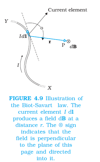
`color {blue}{➢➢}` Figure 4.9 shows a finite conductor `XY` carrying current `I.` Consider an infinitesimal element `dl` of the conductor.
`color{blue} ✍️`The magnetic field `dB` due to this element is to be determined at a point `P` which is at a distance `r` from it. Let `θ` be the angle between `dl` and the displacement vector `r`.
`color{blue} ✍️` According to Biot-Savart’s law, the magnitude of the magnetic field `dB` is proportional to the current `I`, the element length` |dl|,` and inversely proportional to the square of the distance `r`. Its direction* is perpendicular to the plane containing `dl` and r .
Thus, in vector notation,
`color{green}(dB prop (Idlxxr)/(r^3))`
`color {blue}{➢➢}` where `(μ_0)/(4π)` is a constant of proportionality. The above expression holds when the medium is vacuum.
`color {blue}{➢➢}` The magnitude of this field is,
`color {blue}{➢➢}` where we have used the property of cross-product. Equation [4.11 (a)] constitutes our basic equation for the magnetic field. The proportionality constant in SI units has the exact value,
`color {blue}{➢➢}` We call `μ_0` the permeability of free space (or vacuum).
`color{blue} ✍️` The Biot-Savart law for the magnetic field has certain similarities as well as differences with the Coulomb’s law for the electrostatic field. Some of these are:
`color {blue}{(i)}` Both are long range, since both depend inversely on the square of distance from the source to the point of interest.
`color {blue}{➢➢}` The principle of superposition applies to both fields. [In this connection, note that the magnetic field is linear in the source `I dl` just as the electrostatic field is linear in its source: the electric charge.]
`color {blue}{(ii)}` The electrostatic field is produced by a scalar source, namely, the electric charge. The magnetic field is produced by a vector source `I dl.`
`color {blue}{(iii)}` The electrostatic field is along the displacement vector joining the source and the field point. The magnetic field is perpendicular to the plane containing the displacement vector `r` and the current element `I dl.`
`color {blue}{(iv)}`There is an angle dependence in the Biot-Savart law which is not present in the electrostatic case. In Fig. 4.9, the magnetic field at any point in the direction of `dl` (the dashed line) is zero. Along this line, `θ = 0, sin θ = 0` and from Eq. [4.11(a)], `|dB| = 0.`
`color{blue} ✍️` There is an interesting relation between `ε_0,` the permittivity of free spaspace; `μ_0,` the permeability of free space; and `c,` the speed of light in vacuum:
`color{green}(ε_0 μ_0 = (4piε_0) (μ_0 /(4pi)) = (1/(9xx10^9)) (10^(-7)) = 1/(3xx10^8)^2 = 1/(c^2))`
`color{blue} ✍️` We will discuss this connection further in Chapter 8 on the electromagnetic waves. Since the speed of light in vacuum is constant, the product `color{green}(μ_0ε_0)` is fixed in magnitude. Choosing the value of either `ε_0` or `μ_0,` fixes the value of the other. In SI units, `μ_0` is fixed to be equal to `color{green}(4π × 10^(–7))` in magnitude.
`color {blue}{➢➢}` Here, we shall study the relation between current and the magnetic field it produces. It is given by the Biot-Savart’s law.
`color {blue}{➢➢}` Figure 4.9 shows a finite conductor `XY` carrying current `I.` Consider an infinitesimal element `dl` of the conductor.
`color{blue} ✍️`The magnetic field `dB` due to this element is to be determined at a point `P` which is at a distance `r` from it. Let `θ` be the angle between `dl` and the displacement vector `r`.
`color{blue} ✍️` According to Biot-Savart’s law, the magnitude of the magnetic field `dB` is proportional to the current `I`, the element length` |dl|,` and inversely proportional to the square of the distance `r`. Its direction* is perpendicular to the plane containing `dl` and r .
Thus, in vector notation,
`color{green}(dB prop (Idlxxr)/(r^3))`
`color{green}(= (mu_0)/(4pi) (Idlxxr)/(r^3)`
..........[4.11(a)]`color {blue}{➢➢}` where `(μ_0)/(4π)` is a constant of proportionality. The above expression holds when the medium is vacuum.
`color {blue}{➢➢}` The magnitude of this field is,
`color{green}(|dB| = (mu_0)/(4pi) (Idlxxr)/(r^2))`
..........[4.11(b)]`color {blue}{➢➢}` where we have used the property of cross-product. Equation [4.11 (a)] constitutes our basic equation for the magnetic field. The proportionality constant in SI units has the exact value,
`color{green}((mu_0)/(4pi) = 10^(-7) Tm//A)`
...............[4.11(c)]`color {blue}{➢➢}` We call `μ_0` the permeability of free space (or vacuum).
`color{blue} ✍️` The Biot-Savart law for the magnetic field has certain similarities as well as differences with the Coulomb’s law for the electrostatic field. Some of these are:
`color {blue}{(i)}` Both are long range, since both depend inversely on the square of distance from the source to the point of interest.
`color {blue}{➢➢}` The principle of superposition applies to both fields. [In this connection, note that the magnetic field is linear in the source `I dl` just as the electrostatic field is linear in its source: the electric charge.]
`color {blue}{(ii)}` The electrostatic field is produced by a scalar source, namely, the electric charge. The magnetic field is produced by a vector source `I dl.`
`color {blue}{(iii)}` The electrostatic field is along the displacement vector joining the source and the field point. The magnetic field is perpendicular to the plane containing the displacement vector `r` and the current element `I dl.`
`color {blue}{(iv)}`There is an angle dependence in the Biot-Savart law which is not present in the electrostatic case. In Fig. 4.9, the magnetic field at any point in the direction of `dl` (the dashed line) is zero. Along this line, `θ = 0, sin θ = 0` and from Eq. [4.11(a)], `|dB| = 0.`
`color{blue} ✍️` There is an interesting relation between `ε_0,` the permittivity of free spaspace; `μ_0,` the permeability of free space; and `c,` the speed of light in vacuum:
`color{green}(ε_0 μ_0 = (4piε_0) (μ_0 /(4pi)) = (1/(9xx10^9)) (10^(-7)) = 1/(3xx10^8)^2 = 1/(c^2))`
`color{blue} ✍️` We will discuss this connection further in Chapter 8 on the electromagnetic waves. Since the speed of light in vacuum is constant, the product `color{green}(μ_0ε_0)` is fixed in magnitude. Choosing the value of either `ε_0` or `μ_0,` fixes the value of the other. In SI units, `μ_0` is fixed to be equal to `color{green}(4π × 10^(–7))` in magnitude.