`color{blue} ✍️` In the previous chapter, we have explained how a current loop acts as a magnetic dipole (Section 4.10). We mentioned Ampere’s hypothesis that all magnetic phenomena can be explained in terms of circulating currents.
`color {blue}{➢➢}` Recall that the magnetic dipole moment `color{blue}(m)` associated with a current loop was defined to be `color{blue}(m = NI A)` where `color{blue}(N)` is the number of turns in the loop, `color{blue}(I)` the current and `color{blue}(A)` the area vector (Eq. 4.30).
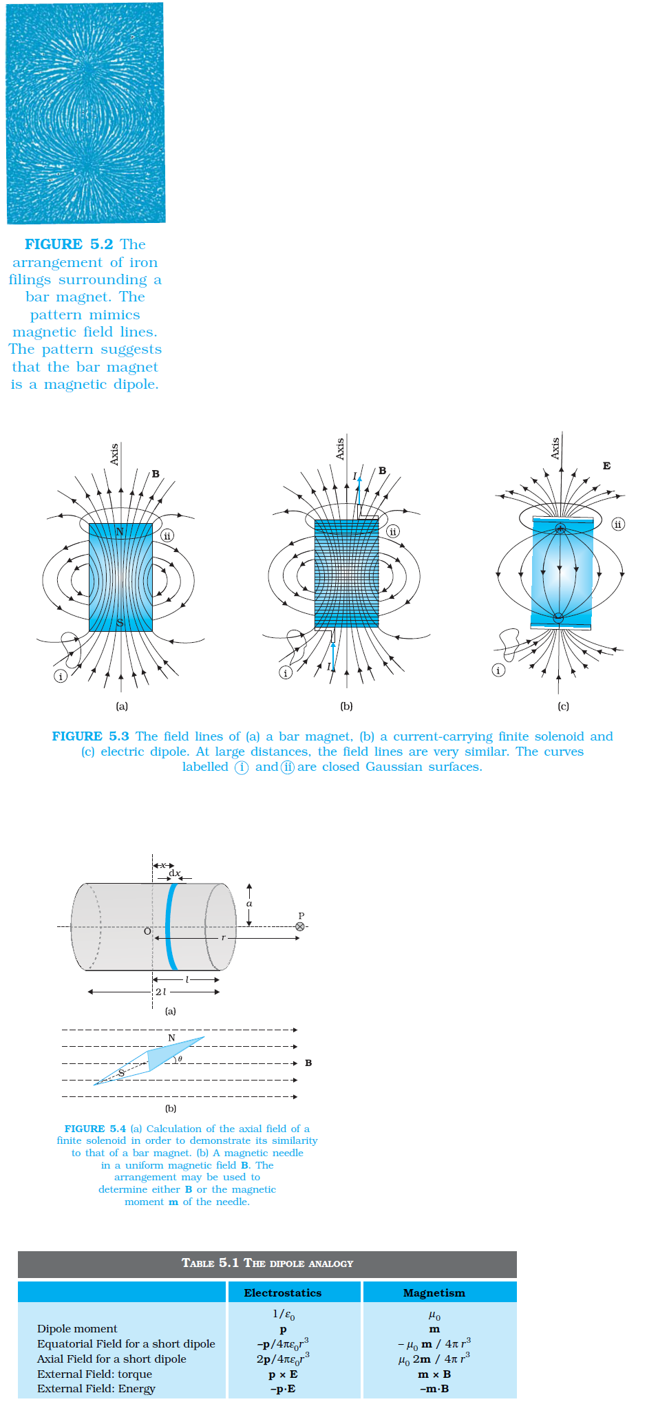
`color{blue} ✍️` The resemblance of magnetic field lines for a bar magnet and a solenoid suggest that a bar magnet may be thought of as a large number of circulating currents in analogy with a solenoid.
`color {blue}{➢➢}` Cutting a bar magnet in half is like cutting a solenoid. We get two smaller solenoids with weaker magnetic properties. The field lines remain continuous, emerging from one face of the solenoid and entering into the other face.
`color {blue}{➢➢}` One can test this analogy by moving a small compass needle in the neighbourhood of a bar magnet and a current-carrying finite solenoid and noting that the deflections of the needle are similar in both cases.
`color {blue}{➢➢}` To make this analogy more firm we calculate the axial field of a finite solenoid depicted in Fig. 5.4 (a). We shall demonstrate that at large distances this axial field resembles that of a bar magnet.

`color{blue} ✍️` Let the solenoid of Fig. 5.4(a) consists of `color{blue}(n)` turns per unit length. Let its length be `color{blue}(2l)` and radius a. We can evaluate the axial field at a point `color{blue}(P)`, at a distance `color{blue}(r)` from the centre `color{blue}(O)` of the solenoid. To do this, consider a circular element of thickness `color{blue}(dx)` of the solenoid at a distance `color{blue}(x)` from its centre. It consists of `color{blue}(n d x)` turns.
`color{blue} ✍️` Let `color{blue}(I)` be the current in the solenoid. In Section 4.6 of the previous chapter we have calculated the magnetic field on the axis of a circular current loop. From Eq. (4.13), the magnitude of the field at point `color{blue}(P)` due to the circular element is
`color{blue}(dB= (mu_0ndxIa^2)/(2[(r-x)^2+a^2]^(3//2)))`
`color {blue}{➢➢}` The magnitude of the total field is obtained by summing over all the elements — in other words by integrating from `color{blue}(x = – l)` to `color{blue}(x = + l)`. Thus,
`color{blue}(B= (mu_0 nla^2)/2 int_(-l)^(l) (dx)/([(r-x)^2+a^2]^(3//2)))`
`color {blue}{➢➢}` This integration can be done by trigonometric substitutions. This exercise, however, is not necessary for our purpose. Note that the range of `color{blue}(x)` is from `color{blue}(– l)` to `color{blue}(+ l)`. Consider the far axial field of the solenoid, i.e., `color{blue}(r > > a)` and `color{blue}(r > > l)` . Then the denominator is approximated by
`color{blue}([(r-x)^2+a^2]^(3//2) approx r^3)`
`color {blue}{➢➢}` and `color{bue}(B = (mu_0 nIa^2)/(2r^3) int_(-l)^(l) dx)`
`color{blue}(= (mu_0 nI)/(2) (2la^2)/(r^3))`
...................(5.1)
`color {brown}bbul{"Note"}` that the magnitude of the magnetic moment of the solenoid is, `color{blue}(m = n (2l) I (πa^2))` — (total number of turns × current × cross-sectional area). Thus,
`color{blue}(B= (mu_0)/(4pi) (2m)/(r^3))`
...............(5.2)
`color {blue}{➢➢}` This is also the far axial magnetic field of a bar magnet which one may obtain experimentally. Thus, a bar magnet and a solenoid produce similar magnetic fields.
`color {blue}{➢➢}` The magnetic moment of a bar magnet is thus equal to the magnetic moment of an equivalent solenoid that produces the same magnetic field.
`color{blue} ✍️`A magnetic charge (also called pole strength) `color{blue}(+q_m)` to the north pole and `color{blue}(–q_m)` to the south pole of a bar magnet of length `color{blue}(2l),` and magnetic moment `color{blue}(q_m(2l )).`
`color {blue}{➢➢}` The field strength due to `color{blue}(q_m)` at a distance r from it is given by `color{blue}(μ_0q_m//4πr^2)`. The magnetic field due to the bar magnet is then obtained, both for the axial and the equatorial case, in a manner analogous to that of an electric dipole.
`color {blue}{➢➢}` The method is simple and appealing. However, magnetic monopoles do not exist, and we have avoided this approach for that reason.
`color{blue} ✍️` In the previous chapter, we have explained how a current loop acts as a magnetic dipole (Section 4.10). We mentioned Ampere’s hypothesis that all magnetic phenomena can be explained in terms of circulating currents.
`color {blue}{➢➢}` Recall that the magnetic dipole moment `color{blue}(m)` associated with a current loop was defined to be `color{blue}(m = NI A)` where `color{blue}(N)` is the number of turns in the loop, `color{blue}(I)` the current and `color{blue}(A)` the area vector (Eq. 4.30).
`color{blue} ✍️` The resemblance of magnetic field lines for a bar magnet and a solenoid suggest that a bar magnet may be thought of as a large number of circulating currents in analogy with a solenoid.
`color {blue}{➢➢}` Cutting a bar magnet in half is like cutting a solenoid. We get two smaller solenoids with weaker magnetic properties. The field lines remain continuous, emerging from one face of the solenoid and entering into the other face.
`color {blue}{➢➢}` One can test this analogy by moving a small compass needle in the neighbourhood of a bar magnet and a current-carrying finite solenoid and noting that the deflections of the needle are similar in both cases.
`color {blue}{➢➢}` To make this analogy more firm we calculate the axial field of a finite solenoid depicted in Fig. 5.4 (a). We shall demonstrate that at large distances this axial field resembles that of a bar magnet.
`color{blue} ✍️` Let the solenoid of Fig. 5.4(a) consists of `color{blue}(n)` turns per unit length. Let its length be `color{blue}(2l)` and radius a. We can evaluate the axial field at a point `color{blue}(P)`, at a distance `color{blue}(r)` from the centre `color{blue}(O)` of the solenoid. To do this, consider a circular element of thickness `color{blue}(dx)` of the solenoid at a distance `color{blue}(x)` from its centre. It consists of `color{blue}(n d x)` turns.
`color{blue} ✍️` Let `color{blue}(I)` be the current in the solenoid. In Section 4.6 of the previous chapter we have calculated the magnetic field on the axis of a circular current loop. From Eq. (4.13), the magnitude of the field at point `color{blue}(P)` due to the circular element is
`color{blue}(dB= (mu_0ndxIa^2)/(2[(r-x)^2+a^2]^(3//2)))`
`color {blue}{➢➢}` The magnitude of the total field is obtained by summing over all the elements — in other words by integrating from `color{blue}(x = – l)` to `color{blue}(x = + l)`. Thus,
`color{blue}(B= (mu_0 nla^2)/2 int_(-l)^(l) (dx)/([(r-x)^2+a^2]^(3//2)))`
`color {blue}{➢➢}` This integration can be done by trigonometric substitutions. This exercise, however, is not necessary for our purpose. Note that the range of `color{blue}(x)` is from `color{blue}(– l)` to `color{blue}(+ l)`. Consider the far axial field of the solenoid, i.e., `color{blue}(r > > a)` and `color{blue}(r > > l)` . Then the denominator is approximated by
`color{blue}([(r-x)^2+a^2]^(3//2) approx r^3)`
`color {blue}{➢➢}` and `color{bue}(B = (mu_0 nIa^2)/(2r^3) int_(-l)^(l) dx)`
`color{blue}(= (mu_0 nI)/(2) (2la^2)/(r^3))`
...................(5.1)
`color {brown}bbul{"Note"}` that the magnitude of the magnetic moment of the solenoid is, `color{blue}(m = n (2l) I (πa^2))` — (total number of turns × current × cross-sectional area). Thus,
`color{blue}(B= (mu_0)/(4pi) (2m)/(r^3))`
...............(5.2)
`color {blue}{➢➢}` This is also the far axial magnetic field of a bar magnet which one may obtain experimentally. Thus, a bar magnet and a solenoid produce similar magnetic fields.
`color {blue}{➢➢}` The magnetic moment of a bar magnet is thus equal to the magnetic moment of an equivalent solenoid that produces the same magnetic field.
`color{blue} ✍️`A magnetic charge (also called pole strength) `color{blue}(+q_m)` to the north pole and `color{blue}(–q_m)` to the south pole of a bar magnet of length `color{blue}(2l),` and magnetic moment `color{blue}(q_m(2l )).`
`color {blue}{➢➢}` The field strength due to `color{blue}(q_m)` at a distance r from it is given by `color{blue}(μ_0q_m//4πr^2)`. The magnetic field due to the bar magnet is then obtained, both for the axial and the equatorial case, in a manner analogous to that of an electric dipole.
`color {blue}{➢➢}` The method is simple and appealing. However, magnetic monopoles do not exist, and we have avoided this approach for that reason.