GROWTH RATES
● The `color{violet}"increased growth"` per unit time is termed as `color{Brown}"growth rate"`.
● Thus, `color{violet}"rate of growth"` can be `color{violet}"expressed mathematically"`.
● An organism, or a `color{violet}"part of the organism"` can produce more cells in a `color{violet}"variety of ways"`.
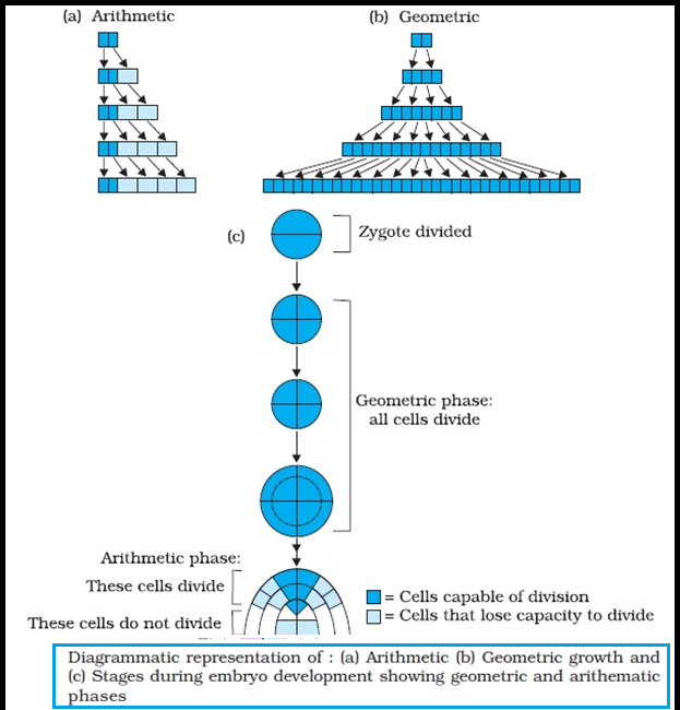
● The `color{violet}"growth rate"` shows an increase that may be `color{vBrown}"arithmetic or geometrical"`.
● In `color{Brown}"arithmetic growth"`, following `color{violet}"mitotic cell division"`, only `color{violet}"one daughter cell"` continues to divide while the `color{violet}"other differentiates"` and matures.
● The `color{violet}"simplest expression"` of arithmetic growth is exemplified by a `color{violet}"root elongating"` at a `color{violet}"constant rate"`.
● On `color{violet}"plotting"` the `color{violet}"length of the organ"` against `color{violet}"time,"` a `color{Brown}"linear curve"` is obtained.
● `color{violet}"Mathematically"`, it is expressed as
`L_t` = `L_0` + `rt`
`L_t` = length at time `t`
`L_0` = length at time ‘zero’
`r` = growth rate / elongation per unit time.

● Let us now see what happens in `color{Brown"geometrical growth"`.
● In `color{violet}"most systems,"` the`color{violet}" initial growth is slow"` (`color{Brown}"lag phase"`), and it `color{violet}"increases rapidly"` thereafter – at an `color{violet}"exponential rate"` (`color{violet}"log or exponential phase"`).
● Here, both the `color{violet}"progeny cells"` following mitotic cell division retain the `color{violet}"ability to divide"` and continue to do so.
● However, `color{violet}"with limited nutrient supply"`, the growth slows down leading to a `color{Brown}"stationary phase"`.
● If we plot the `color{violet}"parameter of growth"` against time, we get a t`color{violet}"ypical"` `color{Brown}"sigmoid or S-curve"`
● A `color{violet}"sigmoid curve"` is a characteristic of `color{violet}"living organism"` growing in a `color{violet}"natural environment"`.
● It is typical for all `color{violet}"cells, tissues"` and `color{violet}"organs of a plant"`.
● The `color{violet}"exponential growth"` can be `color{violet}"expressed"` as
`W_1` = `W_0e^(rt)`
`W_1` = final size (weight, height, number etc.)
`W_0` = initial size at the beginning of the period
`r` = growth rate
`t` = time of growth
`e` = base of natural logarithms
● Here, `color{Brown}"r"` is the `color{violet}"relative growth rate"` and is also the measure of the `color{violet}"ability of the plant"` to produce new plant material, referred to as `color{Brown}"efficiency index"`.
● Hence, the `color{violet}"final size"` of `W_1` depends on the i`color{violet}"nitial size"`, `W_0`.

● `color{violet}"Quantitative comparisons"` between the `color{violet}"growth of living system"` can also be made in two ways :
(i) `color{violet}"Measurement"` and the `color{violet}"comparison"` of total growth per unit time is called the `color{Brown}"absolute growth rate"`.
(ii) The `color{violet}"growth"` of the `color{violet}"given system"` per `color{violet}"unit time"` expressed on a common basis, e.g., per unit initial parameter is called the `color{Brown}"relative growth rate"`.
● In Figure `color{violet}"two leaves,"` `color{vBrown}"A and B,"` are drawn that are of `color{violet}"different sizes"` but shows absolute `color{violet}"increase in area"` in the given time to give `color{violet}"leaves"`, `A_1` and `B_1`.
● However, one of them shows much `color{violet}"higher relative growth rate"`.
● Thus, `color{violet}"rate of growth"` can be `color{violet}"expressed mathematically"`.
● An organism, or a `color{violet}"part of the organism"` can produce more cells in a `color{violet}"variety of ways"`.
● The `color{violet}"growth rate"` shows an increase that may be `color{vBrown}"arithmetic or geometrical"`.
● In `color{Brown}"arithmetic growth"`, following `color{violet}"mitotic cell division"`, only `color{violet}"one daughter cell"` continues to divide while the `color{violet}"other differentiates"` and matures.
● The `color{violet}"simplest expression"` of arithmetic growth is exemplified by a `color{violet}"root elongating"` at a `color{violet}"constant rate"`.
● On `color{violet}"plotting"` the `color{violet}"length of the organ"` against `color{violet}"time,"` a `color{Brown}"linear curve"` is obtained.
● `color{violet}"Mathematically"`, it is expressed as
`L_t` = `L_0` + `rt`
`L_t` = length at time `t`
`L_0` = length at time ‘zero’
`r` = growth rate / elongation per unit time.
● Let us now see what happens in `color{Brown"geometrical growth"`.
● In `color{violet}"most systems,"` the`color{violet}" initial growth is slow"` (`color{Brown}"lag phase"`), and it `color{violet}"increases rapidly"` thereafter – at an `color{violet}"exponential rate"` (`color{violet}"log or exponential phase"`).
● Here, both the `color{violet}"progeny cells"` following mitotic cell division retain the `color{violet}"ability to divide"` and continue to do so.
● However, `color{violet}"with limited nutrient supply"`, the growth slows down leading to a `color{Brown}"stationary phase"`.
● If we plot the `color{violet}"parameter of growth"` against time, we get a t`color{violet}"ypical"` `color{Brown}"sigmoid or S-curve"`
● A `color{violet}"sigmoid curve"` is a characteristic of `color{violet}"living organism"` growing in a `color{violet}"natural environment"`.
● It is typical for all `color{violet}"cells, tissues"` and `color{violet}"organs of a plant"`.
● The `color{violet}"exponential growth"` can be `color{violet}"expressed"` as
`W_1` = `W_0e^(rt)`
`W_1` = final size (weight, height, number etc.)
`W_0` = initial size at the beginning of the period
`r` = growth rate
`t` = time of growth
`e` = base of natural logarithms
● Here, `color{Brown}"r"` is the `color{violet}"relative growth rate"` and is also the measure of the `color{violet}"ability of the plant"` to produce new plant material, referred to as `color{Brown}"efficiency index"`.
● Hence, the `color{violet}"final size"` of `W_1` depends on the i`color{violet}"nitial size"`, `W_0`.
● `color{violet}"Quantitative comparisons"` between the `color{violet}"growth of living system"` can also be made in two ways :
(i) `color{violet}"Measurement"` and the `color{violet}"comparison"` of total growth per unit time is called the `color{Brown}"absolute growth rate"`.
(ii) The `color{violet}"growth"` of the `color{violet}"given system"` per `color{violet}"unit time"` expressed on a common basis, e.g., per unit initial parameter is called the `color{Brown}"relative growth rate"`.
● In Figure `color{violet}"two leaves,"` `color{vBrown}"A and B,"` are drawn that are of `color{violet}"different sizes"` but shows absolute `color{violet}"increase in area"` in the given time to give `color{violet}"leaves"`, `A_1` and `B_1`.
● However, one of them shows much `color{violet}"higher relative growth rate"`.