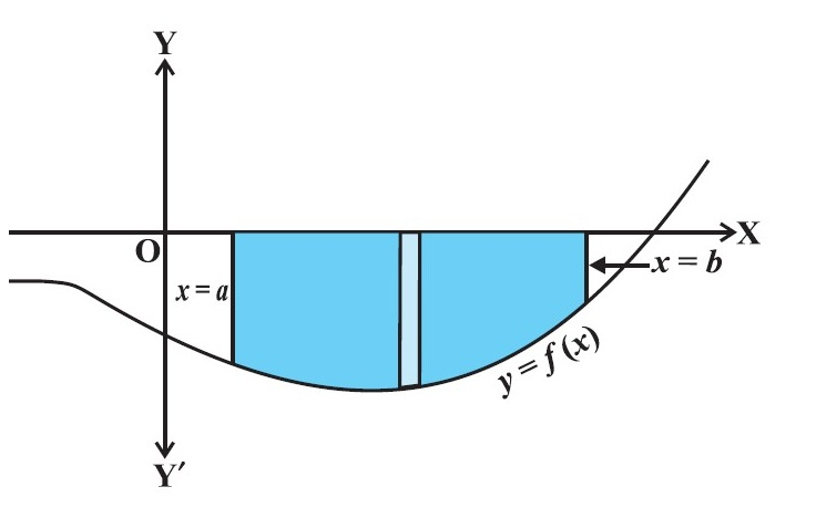
● We can think of area under the curve as composed of large number of very thin vertical strips.
● Consider an arbitrary strip of height `y` and width `color{blue}{dx}`,
`color{green} ✍️ color{red}{dA "(area of the elementary strip)"= ydx, }` where, y = f (x).
● Total area `A` of the region between x-axis, ordinates `x = a, x = b` and the curve `y = f (x)` as the result of adding up the elementary areas of thin strips across the region PQRSP. Symbolically, we express
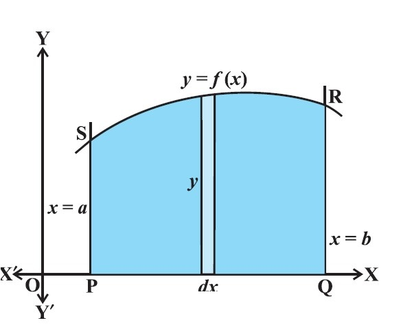
● Here, we consider vertical strips as shown in the Fig
`color{blue} {A = int_a^b d A = int_a^b ydx = int_a^b f(x) dx}`
● The area A of the region bounded by the curve `x = g (y), y`-axis and the lines `y = c, y = d` is given by
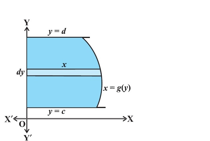
● Here, we consider horizontal strips as shown in the Fig
`color{blue} {A = int_c^d x dy = int_c^d g(y) dy}`
● We can think of area under the curve as composed of large number of very thin vertical strips.
● Consider an arbitrary strip of height `y` and width `color{blue}{dx}`,
`color{green} ✍️ color{red}{dA "(area of the elementary strip)"= ydx, }` where, y = f (x).
● Total area `A` of the region between x-axis, ordinates `x = a, x = b` and the curve `y = f (x)` as the result of adding up the elementary areas of thin strips across the region PQRSP. Symbolically, we express
● Here, we consider vertical strips as shown in the Fig
`color{blue} {A = int_a^b d A = int_a^b ydx = int_a^b f(x) dx}`
● The area A of the region bounded by the curve `x = g (y), y`-axis and the lines `y = c, y = d` is given by
● Here, we consider horizontal strips as shown in the Fig
`color{blue} {A = int_c^d x dy = int_c^d g(y) dy}`