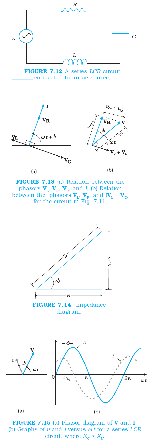
`color{blue} ✍️`Figure 7.12 shows a series LCR circuit connected to an ac source e. As usual, we take the voltage of the source to be `v = v_m sin omega t.`
`color {blue}{➢➢}`If q is the charge on the capacitor and i the current, at time t, we have, from Kirchhoff’s loop rule:
`color{green}(L (di)/(dt) +i R + q/C =v)`
.............(7.20)
`color{blue} ✍️`We want to determine the instantaneous current i and its phase relationship to the applied alternating voltage v. We shall solve this problem by two methods. First, we use the technique of phasors and in the second method, we solve Eq. (7.20) analytically to obtain the time– dependence of `i` .
`color{green}bbul("Phasor-diagram solution")`
`color {blue}{➢➢}`From the circuit shown in Fig. 7.12, we see that the resistor, inductor and capacitor are in series. Therefore, the ac current in each element is the same at any time, having the same amplitude and phase. Let it be
`color{green}(i = i_m sin(omegat + phi))`
............(7.21)
`color {blue}{➢➢}`where `phi` is the phase difference between the voltage across the source and the current in the circuit. On the basis of what we have learnt in the previous
sections, we shall construct a phasor diagram for the present case.

`color{blue} ✍️`Let `I` be the phasor representing the current in the circuit as given by Eq. (7.21). Further, let `color{green}(V_L, V_R, V_C,)` and V represent the voltage across the inductor, resistor, capacitor and the source, respectively. From previous section, we know that `V_R` is parallel to `color{green}(I, V_C)` is `color{green}(pi//2)` behind I and `color{green}(V_L)` is `color{green}(pi//2)` ahead of `color{green}(I. V_L, V_R, V_C)` and `I` are shown in Fig. 7.13(a) with appropriate phase relations.
`color {blue}{➢➢}`The length of these phasors or the amplitude of `color{green}(V_R V_C)` and `V_L` are;
`color{green}(v_(Rm) = i_m R, v_(Cm) = i_m X_C v_(Lm) = i_m X_L)`
..........(7.22)
`color {blue}{➢➢}`The voltage Equation (7.20) for the circuit can be written as
`color{green}(v_L +v_R v_C =v)`
..............(7.23)
`color {blue}{➢➢}`The phasor relation whose vertical component gives the above equation is
`color{green}(V_L +V_R V_C =v)`
............(7.24)
`color {blue}{➢➢}`This relation is represented in Fig. 7.13(b).
`color {blue}{➢➢}`Since `V_C` and `V_L` are always along the same line and in opposite directions, they can be combined into a single phasor `color{green}((V_C + V_L))` which has a magnitude `color{green}(|v_(Cm) – v_(Lm)|)`.
`color {blue}{➢➢}`Since `V` is represented as the hypotenuse of a right-traingle whose sides are `V_R` and `color{green}((VC + VL)),` the pythagorean theorem gives:
`color{green}(v_(m)^(2) = v_(Rm)^(2) + (v_(Cm) - v_(Lm)^2)`
`color {blue}{➢➢}`Substituting the values of `v_(Rm), v_(Cm,)` and `v_(Lm)` from Eq. (7.22) into the above equation, we have
`color{green}(v_(m)^(2) = (i_mR)^2+(i_mX_C-i_mX_L)^2)`
`color{green}(= i_(m)^(i) [ R^2+(X_C-X_L)^2])`
or
`color{green}(i_m = (v_m)/(sqrtR^2 + (X_C-X_L)^2))`
............[7.25(a)]
`color {blue}{➢➢}`By analogy to the resistance in a circuit, we introduce the impedance Z in an ac circuit:
`color{green}(i_m = (v_m))`
............[7.25(b)]
`color {blue}{➢➢}`where
`color{green}(Z = sqrt(R^2+(X_C-X_L)^2))`
...........(7.26)
`color {blue}{➢➢}`Since phasor `I` is always parallel to phasor `V_R` . the phase angle `phi` is the angle between `V_R` and `V` and can be determined from
Fig. 7.14:
` tan phi = (v_(Cm) - v_(Lm))/(v_(Rm)`
`color {blue}{➢➢}` Using Eq. (7.22), we have
` tan phi = (X_C - X_L)/R`
.............(7.27)

`color {blue}{➢➢}`Equations (7.26) and (7.27) are graphically shown in Fig. (7.14). This is called Impedance diagram which is a right-triangle with Z as its hypotenuse.
`color {blue}{➢➢}`Equation 7.25(a) gives the amplitude of the current and Eq. (7.27) gives the phase angle. With these, Eq. (7.21) is completely specified
`color {blue}{➤➤}`If `X_C > X_L , phi` is positive and the circuit is predominantly capacitive. Consequently, the current in the circuit leads the source voltage.
`color {blue}{➤➤}`If `X_C < X_L , phi` is negative and the circuit is predominantly inductive. Consequently, the current in the circuit lags the source voltage.

`color {blue}{➢➢}`Figure 7.15 shows the phasor diagram and variation of v and i with `ω t` for the case `X_C > X_L`.
`color {blue}{➢➢}`Thus, we have obtained the amplitude and phase of current for an LCR series circuit using the technique of phasors. But this method of analysing ac circuits suffers from certain disadvantages.
First, the phasor diagram say nothing about the initial condition. One can take any arbitrary value of t (say, `t_1`, as done throughout this chapter) and draw different phasors which show the relative angle between different phasors.
`color {blue}{➢➢}`The solution so obtained is called the steady-state solution. This is not a general solution. Additionally, we do have a transient solution which exists even for `v = 0`. The general solution is the sum of the transient solution and the steady-state solution.
After a sufficiently long time, the effects of the transient solution die out and the behaviour of the circuit is described by the steady-state solution
`color{brown}bbul("Analytical solution")`
The voltage equation for the circuit is `color{green}(L(di)/(dt) +Ri + q/c =v)`
`=color{green}(v_m sin omegat)`
`color {blue}{➢➢}`We know that `color{green}(i = dq//dt.)` Therefore, `color{green}((di)/dt = (d^2q)/dt^2)`. Thus, in terms of `q,` the voltage equation becomes
`color{green}(L(d^2q)/(dt^2) + (R_dp)/(dt) + q/c= v_m sin omegat)`
.........(7.28)
This is like the equation for a forced, damped oscillator, [see Eq. {14.37(b)} in Class XI Physics Textbook]. Let us assume a solution
`color{green}(q = q_m sin (omegay+theta))`
..........[7.29(a)]
`color {blue}{➢➢}`so that `color{green}((dp)/(dt) = q_m omega cos (omegat+theta))`
..........[7.29(b)]
and
`color{green}((d^2q)/(dt^2) = - q_m omega^2 sin (omegat+theta))`
..........[7.29(c)]
`color {blue}{➢➢}`Substituting these values in Eq. (7.28), we get
`color{green}(q_m omega[R cos (omegat+theta) + (X_C - X_L ) sin (omegat+theta) = v_m sin omega t)`
...........(7.30)
`color {blue}{➢➢}`where we have used the relation `color{green}(X_c= 1//omegaC, X_L = omega L.)` Multiplying and
dividing Eq. (7.30) by `color{green}(Z = sqrt(R^2+(X_C-X_L)^2)` we have
`color{green}(q_m omegaZ [R/Z cos (omegat+theta) + (X_C-X_L)/Z sin (omegat+theta)] = v_m sin omegat)`
.........(7.31)
`color {blue}{➢➢}`Now, let `color{green}(R/Z = cos phi)`
and `color{green}((X_C-X_L)/Z = sin phi)`
`color{green}(phi = tan^(-1) " " (X_C-X_L)/R)`
...........(7.32)
`color {blue}{➢➢}`Substituting this in Eq. (7.31) and simplifying, we get:
`color{green}(q_m omegaZcos (omegat+theta-phi) = v_m sin omegat)`
............(7.33)
`color {blue}{➢➢}`Comparing the two sides of this equation, we see that
`color{green}(v_m = q_m omegaZ= i_m Z)`
`color {blue}{➢➢}`where `color{green}(i_m = q_m omega)`.........[7.33(a)]
`color {blue}{➢➢}`and
`color{green}(theta phi = pi /2 or theta =- pi/2 + phi)`
..........[7.33(b)]
`color {blue}{➢➢}`Therefore, the current in the circuit is
`color{green}(i = (dq)/(dt) = q_m cos (omegat + theta))`
`color{green}(= i_m cos(omegat+theta))`
or
`color{green}(i = i_m sin (omega t+phi))`
..........(7.34)
`color {blue}{➢➢}`where
`color{green}(i_m = (v_m)/Z = (v_m)/(sqrt(R^2+(X_C-X_L)^2))`
.............[7.34(a)]
`color {blue}{➢➢}`and `color{green}(phi = tan^(-1) ((X_X-X_L)/(R)))`
`color {blue}{➢➢}`Thus, the analytical solution for the amplitude and phase of the current in the circuit agrees with that obtained by the technique of phasors.
`color{blue} ✍️`Figure 7.12 shows a series LCR circuit connected to an ac source e. As usual, we take the voltage of the source to be `v = v_m sin omega t.`
`color {blue}{➢➢}`If q is the charge on the capacitor and i the current, at time t, we have, from Kirchhoff’s loop rule:
`color{green}(L (di)/(dt) +i R + q/C =v)`
.............(7.20)
`color{blue} ✍️`We want to determine the instantaneous current i and its phase relationship to the applied alternating voltage v. We shall solve this problem by two methods. First, we use the technique of phasors and in the second method, we solve Eq. (7.20) analytically to obtain the time– dependence of `i` .
`color{green}bbul("Phasor-diagram solution")`
`color {blue}{➢➢}`From the circuit shown in Fig. 7.12, we see that the resistor, inductor and capacitor are in series. Therefore, the ac current in each element is the same at any time, having the same amplitude and phase. Let it be
`color{green}(i = i_m sin(omegat + phi))`
............(7.21)
`color {blue}{➢➢}`where `phi` is the phase difference between the voltage across the source and the current in the circuit. On the basis of what we have learnt in the previous
sections, we shall construct a phasor diagram for the present case.
`color{blue} ✍️`Let `I` be the phasor representing the current in the circuit as given by Eq. (7.21). Further, let `color{green}(V_L, V_R, V_C,)` and V represent the voltage across the inductor, resistor, capacitor and the source, respectively. From previous section, we know that `V_R` is parallel to `color{green}(I, V_C)` is `color{green}(pi//2)` behind I and `color{green}(V_L)` is `color{green}(pi//2)` ahead of `color{green}(I. V_L, V_R, V_C)` and `I` are shown in Fig. 7.13(a) with appropriate phase relations.
`color {blue}{➢➢}`The length of these phasors or the amplitude of `color{green}(V_R V_C)` and `V_L` are;
`color{green}(v_(Rm) = i_m R, v_(Cm) = i_m X_C v_(Lm) = i_m X_L)`
..........(7.22)
`color {blue}{➢➢}`The voltage Equation (7.20) for the circuit can be written as
`color{green}(v_L +v_R v_C =v)`
..............(7.23)
`color {blue}{➢➢}`The phasor relation whose vertical component gives the above equation is
`color{green}(V_L +V_R V_C =v)`
............(7.24)
`color {blue}{➢➢}`This relation is represented in Fig. 7.13(b).
`color {blue}{➢➢}`Since `V_C` and `V_L` are always along the same line and in opposite directions, they can be combined into a single phasor `color{green}((V_C + V_L))` which has a magnitude `color{green}(|v_(Cm) – v_(Lm)|)`.
`color {blue}{➢➢}`Since `V` is represented as the hypotenuse of a right-traingle whose sides are `V_R` and `color{green}((VC + VL)),` the pythagorean theorem gives:
`color{green}(v_(m)^(2) = v_(Rm)^(2) + (v_(Cm) - v_(Lm)^2)`
`color {blue}{➢➢}`Substituting the values of `v_(Rm), v_(Cm,)` and `v_(Lm)` from Eq. (7.22) into the above equation, we have
`color{green}(v_(m)^(2) = (i_mR)^2+(i_mX_C-i_mX_L)^2)`
`color{green}(= i_(m)^(i) [ R^2+(X_C-X_L)^2])`
or
`color{green}(i_m = (v_m)/(sqrtR^2 + (X_C-X_L)^2))`
............[7.25(a)]
`color {blue}{➢➢}`By analogy to the resistance in a circuit, we introduce the impedance Z in an ac circuit:
`color{green}(i_m = (v_m))`
............[7.25(b)]
`color {blue}{➢➢}`where
`color{green}(Z = sqrt(R^2+(X_C-X_L)^2))`
...........(7.26)
`color {blue}{➢➢}`Since phasor `I` is always parallel to phasor `V_R` . the phase angle `phi` is the angle between `V_R` and `V` and can be determined from
Fig. 7.14:
` tan phi = (v_(Cm) - v_(Lm))/(v_(Rm)`
`color {blue}{➢➢}` Using Eq. (7.22), we have
` tan phi = (X_C - X_L)/R`
.............(7.27)
`color {blue}{➢➢}`Equations (7.26) and (7.27) are graphically shown in Fig. (7.14). This is called Impedance diagram which is a right-triangle with Z as its hypotenuse.
`color {blue}{➢➢}`Equation 7.25(a) gives the amplitude of the current and Eq. (7.27) gives the phase angle. With these, Eq. (7.21) is completely specified
`color {blue}{➤➤}`If `X_C > X_L , phi` is positive and the circuit is predominantly capacitive. Consequently, the current in the circuit leads the source voltage.
`color {blue}{➤➤}`If `X_C < X_L , phi` is negative and the circuit is predominantly inductive. Consequently, the current in the circuit lags the source voltage.
`color {blue}{➢➢}`Figure 7.15 shows the phasor diagram and variation of v and i with `ω t` for the case `X_C > X_L`.
`color {blue}{➢➢}`Thus, we have obtained the amplitude and phase of current for an LCR series circuit using the technique of phasors. But this method of analysing ac circuits suffers from certain disadvantages.
First, the phasor diagram say nothing about the initial condition. One can take any arbitrary value of t (say, `t_1`, as done throughout this chapter) and draw different phasors which show the relative angle between different phasors.
`color {blue}{➢➢}`The solution so obtained is called the steady-state solution. This is not a general solution. Additionally, we do have a transient solution which exists even for `v = 0`. The general solution is the sum of the transient solution and the steady-state solution.
After a sufficiently long time, the effects of the transient solution die out and the behaviour of the circuit is described by the steady-state solution
`color{brown}bbul("Analytical solution")`
The voltage equation for the circuit is `color{green}(L(di)/(dt) +Ri + q/c =v)`
`=color{green}(v_m sin omegat)`
`color {blue}{➢➢}`We know that `color{green}(i = dq//dt.)` Therefore, `color{green}((di)/dt = (d^2q)/dt^2)`. Thus, in terms of `q,` the voltage equation becomes
`color{green}(L(d^2q)/(dt^2) + (R_dp)/(dt) + q/c= v_m sin omegat)`
.........(7.28)
This is like the equation for a forced, damped oscillator, [see Eq. {14.37(b)} in Class XI Physics Textbook]. Let us assume a solution
`color{green}(q = q_m sin (omegay+theta))`
..........[7.29(a)]
`color {blue}{➢➢}`so that `color{green}((dp)/(dt) = q_m omega cos (omegat+theta))`
..........[7.29(b)]
and
`color{green}((d^2q)/(dt^2) = - q_m omega^2 sin (omegat+theta))`
..........[7.29(c)]
`color {blue}{➢➢}`Substituting these values in Eq. (7.28), we get
`color{green}(q_m omega[R cos (omegat+theta) + (X_C - X_L ) sin (omegat+theta) = v_m sin omega t)`
...........(7.30)
`color {blue}{➢➢}`where we have used the relation `color{green}(X_c= 1//omegaC, X_L = omega L.)` Multiplying and
dividing Eq. (7.30) by `color{green}(Z = sqrt(R^2+(X_C-X_L)^2)` we have
`color{green}(q_m omegaZ [R/Z cos (omegat+theta) + (X_C-X_L)/Z sin (omegat+theta)] = v_m sin omegat)`
.........(7.31)
`color {blue}{➢➢}`Now, let `color{green}(R/Z = cos phi)`
and `color{green}((X_C-X_L)/Z = sin phi)`
`color{green}(phi = tan^(-1) " " (X_C-X_L)/R)`
...........(7.32)
`color {blue}{➢➢}`Substituting this in Eq. (7.31) and simplifying, we get:
`color{green}(q_m omegaZcos (omegat+theta-phi) = v_m sin omegat)`
............(7.33)
`color {blue}{➢➢}`Comparing the two sides of this equation, we see that
`color{green}(v_m = q_m omegaZ= i_m Z)`
`color {blue}{➢➢}`where `color{green}(i_m = q_m omega)`.........[7.33(a)]
`color {blue}{➢➢}`and
`color{green}(theta phi = pi /2 or theta =- pi/2 + phi)`
..........[7.33(b)]
`color {blue}{➢➢}`Therefore, the current in the circuit is
`color{green}(i = (dq)/(dt) = q_m cos (omegat + theta))`
`color{green}(= i_m cos(omegat+theta))`
or
`color{green}(i = i_m sin (omega t+phi))`
..........(7.34)
`color {blue}{➢➢}`where
`color{green}(i_m = (v_m)/Z = (v_m)/(sqrt(R^2+(X_C-X_L)^2))`
.............[7.34(a)]
`color {blue}{➢➢}`and `color{green}(phi = tan^(-1) ((X_X-X_L)/(R)))`
`color {blue}{➢➢}`Thus, the analytical solution for the amplitude and phase of the current in the circuit agrees with that obtained by the technique of phasors.