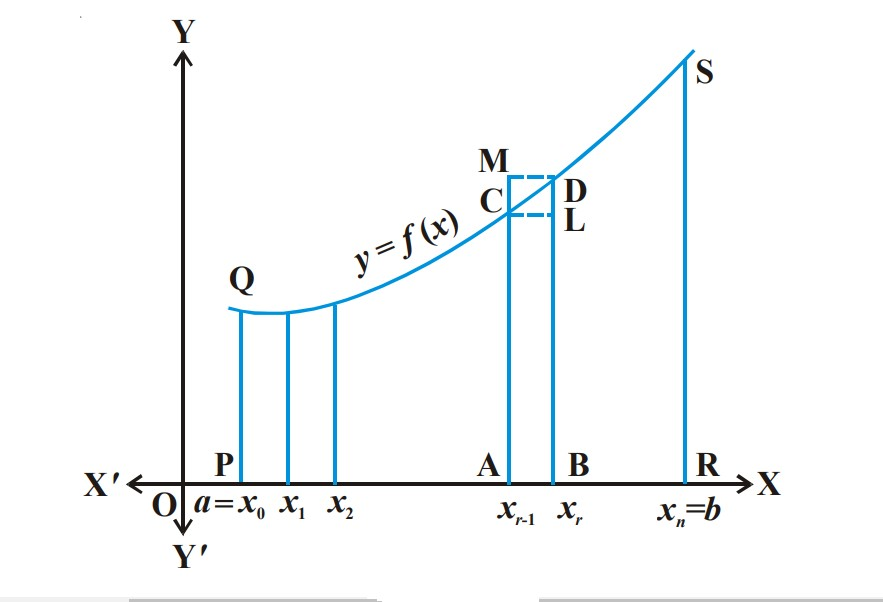
`=>` To evaluate this area, consider the region PRSQP between this curve, x-axis and the ordinates `x = a` and `x = b.`
`=>1.` Divide the interval `[a, b]` into `n` equal subintervals denoted by `[x_0, x_1], [x_1,x_2] ,...., [x_(r-1), x_r],..., [x_(n-1), x_n]`, where `x_0 = a, x_1 = a + h, x_2 = a +2h, ..., x_r = a + rh` and `x_n = b = a + nh` or `n = (b-a)/h`. We note that as n → ∞, h → 0.
`=>2.` The region `PRSQP` under consideration is the sum of `n` subregions, where each subregion is defined on subintervals `[x_(r-1), x_r] , r =1,2,3 ...n`
From Fig `=>`
`=>color{green}{"Area of the rectangle (ABLC) < area of the region (ABDCA) < area of the rectangle (ABDM)"}`
`=>3.` Evidently as `x_r – x_(r–1 )→ 0`, i.e., h → 0 all the three areas shown in (1) become nearly equal to each other. Now we form the following sums.
`color{brown}{s_n = h [f(x_0) + ..... + f(x_(n-1) )] = h sum_(r=0)^(n-1) f(x_r)}`........(2)
and `color{brown} {S_n = h[ f(x_1) +f(x_2) +......+ f(x_n)] = h sum_(r=1)^n f(x_r)}`........(3)
`=>4.` Here, `s_n` and `S_n` denote the sum of areas of all lower rectangles and upper rectangles raised over sub intervals `[x_(r–1), x_r]` for r = 1, 2, 3, …, n, respectively.
In view of the inequality (1) for an arbitrary subinterval `[x_(r-1), x_r]` ,we have
`color{blue}{=>}` `s_n` < area of the region PRSQP < `S_n`
`=>` As `n -> oo` strips become narrower and narrower, it is assumed that the limiting values of (2) and (3) are the same in both cases and the common limiting value is the required area under the curve.
Symbolically, we write
`color{orange}{lim_(n->oo) S_n = lim_(n->oo) s_n = "area of the region PRSQP "= int_a^b f(x) dx}` ... (5)
`=>5. ` It follows that this area is also the limiting value of any area which is between that of the rectangles below the curve and that of the rectangles above the curve.
`=>` For the sake of convenience, we shall take rectangles with height equal to that of the curve at the left hand edge of each subinterval. Thus, we rewrite (5) as
`color {brown} {int_a^b f(x) dx = lim_(h ->0) h [ f(a) + f(a +h) +....+ f(a + (n -1) h ]}`
or ` int_a^b f(x) dx = (b -a) lim_(n -> oo) 1/n [ f(a) + f(a +h) +.... + f(a + ( n-1) h ]` ......(6)
where `h = (b -a)/n -> 0` as `n-> oo`
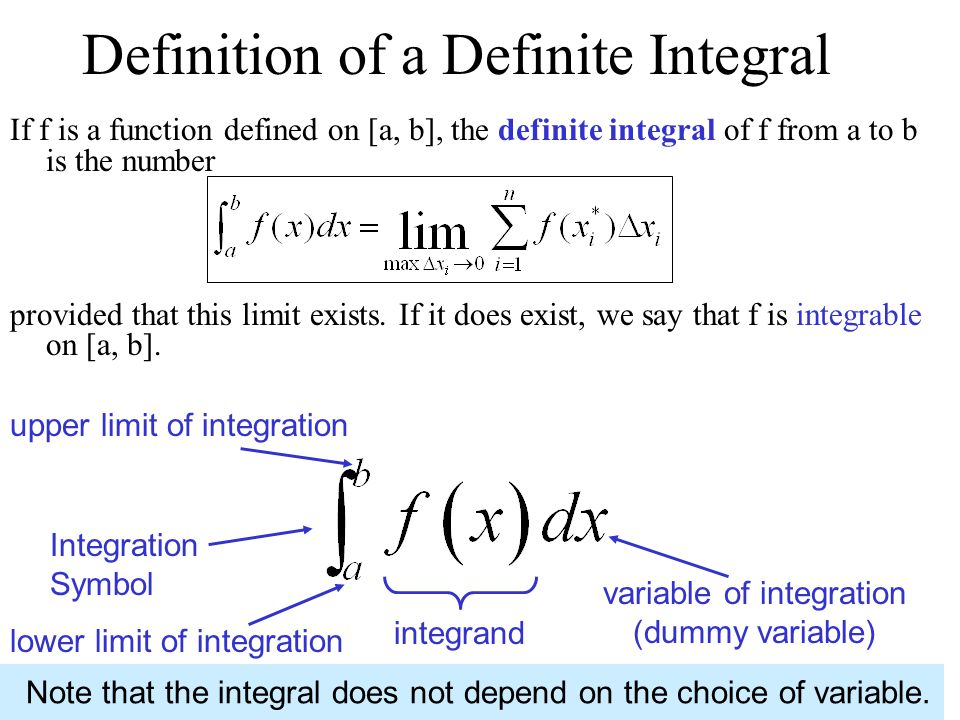
The above expression (6) is known as the definition of definite integral as the limit of sum.
`color {blue} text{Remarks}`
`=>`The value of the definite integral of a function over any particular interval depends on the function and the interval, but not on the variable of integration that we choose to represent the independent variable. If the independent variable is denoted by t or u instead of x, we simply write the integral as ` int_a^b f(t) dt` or `int_a^b f(u) du` instead of `int_a^b f(x) dx`. Hence, the the variable of integration is called a dummy variable.
`=>` To evaluate this area, consider the region PRSQP between this curve, x-axis and the ordinates `x = a` and `x = b.`
`=>1.` Divide the interval `[a, b]` into `n` equal subintervals denoted by `[x_0, x_1], [x_1,x_2] ,...., [x_(r-1), x_r],..., [x_(n-1), x_n]`, where `x_0 = a, x_1 = a + h, x_2 = a +2h, ..., x_r = a + rh` and `x_n = b = a + nh` or `n = (b-a)/h`. We note that as n → ∞, h → 0.
`=>2.` The region `PRSQP` under consideration is the sum of `n` subregions, where each subregion is defined on subintervals `[x_(r-1), x_r] , r =1,2,3 ...n`
From Fig `=>`
`=>color{green}{"Area of the rectangle (ABLC) < area of the region (ABDCA) < area of the rectangle (ABDM)"}`
`=>3.` Evidently as `x_r – x_(r–1 )→ 0`, i.e., h → 0 all the three areas shown in (1) become nearly equal to each other. Now we form the following sums.
`color{brown}{s_n = h [f(x_0) + ..... + f(x_(n-1) )] = h sum_(r=0)^(n-1) f(x_r)}`........(2)
and `color{brown} {S_n = h[ f(x_1) +f(x_2) +......+ f(x_n)] = h sum_(r=1)^n f(x_r)}`........(3)
`=>4.` Here, `s_n` and `S_n` denote the sum of areas of all lower rectangles and upper rectangles raised over sub intervals `[x_(r–1), x_r]` for r = 1, 2, 3, …, n, respectively.
In view of the inequality (1) for an arbitrary subinterval `[x_(r-1), x_r]` ,we have
`color{blue}{=>}` `s_n` < area of the region PRSQP < `S_n`
`=>` As `n -> oo` strips become narrower and narrower, it is assumed that the limiting values of (2) and (3) are the same in both cases and the common limiting value is the required area under the curve.
Symbolically, we write
`color{orange}{lim_(n->oo) S_n = lim_(n->oo) s_n = "area of the region PRSQP "= int_a^b f(x) dx}` ... (5)
`=>5. ` It follows that this area is also the limiting value of any area which is between that of the rectangles below the curve and that of the rectangles above the curve.
`=>` For the sake of convenience, we shall take rectangles with height equal to that of the curve at the left hand edge of each subinterval. Thus, we rewrite (5) as
`color {brown} {int_a^b f(x) dx = lim_(h ->0) h [ f(a) + f(a +h) +....+ f(a + (n -1) h ]}`
or ` int_a^b f(x) dx = (b -a) lim_(n -> oo) 1/n [ f(a) + f(a +h) +.... + f(a + ( n-1) h ]` ......(6)
where `h = (b -a)/n -> 0` as `n-> oo`
The above expression (6) is known as the definition of definite integral as the limit of sum.
`color {blue} text{Remarks}`
`=>`The value of the definite integral of a function over any particular interval depends on the function and the interval, but not on the variable of integration that we choose to represent the independent variable. If the independent variable is denoted by t or u instead of x, we simply write the integral as ` int_a^b f(t) dt` or `int_a^b f(u) du` instead of `int_a^b f(x) dx`. Hence, the the variable of integration is called a dummy variable.